Page 431 - Mechanical Engineers' Handbook (Volume 2)

422 Basic Control Systems Design

Figure 42 (a) Root-locus plot for s(s 1)(s 2) K 0, for K 0. (b) The effect of PD control
2
with T D ⁄3.

Ks K I
P
T (s) (42)
1
2
3
s as (a K )s K I
2
1
P
Note that the Ziegler–Nichols rules cannot be used to set the gains K and K . The second-
I
P
order plant, Eq. (41), does not have the S-shaped signature of Fig. 33, so the process reaction
method does not apply. The ultimate-cycle method requires K to be set to zero and the
I
ultimate gain K Pu determined. With K 0 in Eq. (42) the resulting system is stable for all
I
K 0, and thus a positive ultimate gain does not exist.
P
Take the form of the PI control law given by Eq. (42) with T 0, and assume that
D
the characteristic roots of the plant (Fig. 44) are real values r and r such that r
2
1
2
r . In this case the open-loop transfer function of the control system is
1

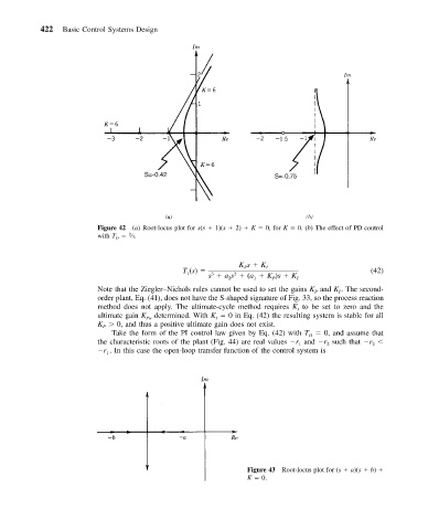
Figure 43 Root-locus plot for (s a)(s b)
K 0.