Page 434 - Mechanical Engineers' Handbook (Volume 2)

10 Principles of Digital Control 425

10.1 Digital Controller Structure
Sampling, discrete-time models, the z-transform, and pulse transfer functions were outlined
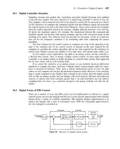
in the previous chapter. The basic structure of a single-loop controller is shown in Fig. 46.
The computer with its internal clock drives the digital-to-analog (D/A) and analog-to-digital
(A/D) converters. It compares the command signals with the feedback signals and generates
the control signals to be sent to the final control elements. These control signals are computed
from the control algorithm stored in the memory. Slightly different structures exist, but Fig.
46 shows the important aspects. For example, the comparison between the command and
feedback signals can be done with analog elements, and the A/D conversion made on the
resulting error signal. The software must also provide for interrupts, which are conditions
that call for the computer’s attention to do something other than computing the control
algorithm.
The time required for the control system to complete one loop of the algorithm is the
time T, the sampling time of the control system. It depends on the time required for the
computer to calculate the control algorithm and on the time required for the interfaces to
convert data. Modern systems are capable of very high rates, with sample times under 1
s.
In most digital control applications, the plant is an analog system, but the controller is
a discrete-time system. Thus, to design a digital control system, we must either model the
controller as an analog system or model the plant as a discrete-time system. Each approach
has its own merits, and we will examine both.
If we model the controller as an analog system, we use methods based on differential
equations to compute the gains. However, a digital control system requires difference equa-
tions to describe its behavior. Thus, from a strictly mathematical point of view, the gain
values we will compute will not give the predicted response exactly. However, if the sampling
time is small compared to the smallest time constant in the system, then the digital system
will act like an analog system, and our designs will work properly. Because most physical
systems of interest have time constants greater than 1 ms and controllers can now achieve
sampling times less than 1
s, controllers designed with analog methods will often be ad-
equate.

10.2 Digital Forms of PID Control
There are a number of ways that PID control can be implemented in software in a digital
control system, because the integral and derivative terms must be approximated with formulas
chosen from a variety of available algorithms. The simplest integral approximation is to
replace the integral with a sum of rectangular areas. With this rectangular approximation,
the error integral is calculated as

Figure 46 Structure of a digital control system. 1