Page 740 - Mechanical Engineers' Handbook (Volume 2)

3 State-Variable Selection and Canonical Forms 731

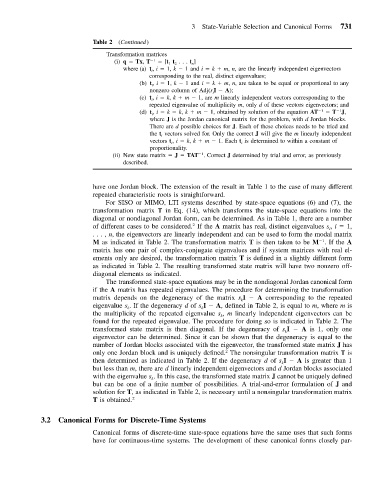
Table 2 (Continued)
Transformation matrices
(i) q Tx, T 1 [t 1 t 2 .. . t n ]
where (a) t i , i 1, k 1 and i k m, n, are the linearly independent eigenvectors
corresponding to the real, distinct eigenvalues;
(b) t i , i 1, k 1 and i k m, n, are taken to be equal or proportional to any
nonzero column of Adj(s i I A);
(c) t i , i k, k m 1, are m linearly independent vectors corresponding to the
repeated eigenvalue of multiplicity m, only d of these vectors eigenvectors; and
(d) t i , i k k, k m 1, obtained by solution of the equation AT 1 T J,
1
where J is the Jordan canonical matrix for the problem, with d Jordan blocks.
There are d possible choices for J. Each of these choices needs to be tried and
the t i vectors solved for. Only the correct J will give the m linearly independent
vectors t i , i k, k m 1. Each t i is determined to within a constant of
proportionality.
(ii) New state matrix J TAT . Correct J determined by trial and error, as previously
1
described.

have one Jordan block. The extension of the result in Table 1 to the case of many different
repeated characteristic roots is straightforward.
For SISO or MIMO, LTI systems described by state-space equations (6) and (7), the
transformation matrix T in Eq. (14), which transforms the state-space equations into the
diagonal or nondiagonal Jordan form, can be determined. As in Table 1, there are a number
of different cases to be considered. If the A matrix has real, distinct eigenvalues s , i 1,
2
i
..., n, the eigenvectors are linearly independent and can be used to form the modal matrix
M as indicated in Table 2. The transformation matrix T is then taken to be M .Ifthe A
1
matrix has one pair of complex-conjugate eigenvalues and if system matrices with real el-
ements only are desired, the transformation matrix T is defined in a slightly different form
as indicated in Table 2. The resulting transformed state matrix will have two nonzero off-
diagonal elements as indicated.
The transformed state-space equations may be in the nondiagonal Jordan canonical form
if the A matrix has repeated eigenvalues. The procedure for determining the transformation
matrix depends on the degeneracy of the matrix s I A corresponding to the repeated
k
eigenvalue s . If the degeneracy d of s I A,defined in Table 2, is equal to m, where m is
k
k
the multiplicity of the repeated eigenvalue s , m linearly independent eigenvectors can be
k
found for the repeated eigenvalue. The procedure for doing so is indicated in Table 2. The
transformed state matrix is then diagonal. If the degeneracy of s I A is 1, only one
k
eigenvector can be determined. Since it can be shown that the degeneracy is equal to the
number of Jordan blocks associated with the eigenvector, the transformed state matrix J has
2
only one Jordan block and is uniquely defined. The nonsingular transformation matrix T is
then determined as indicated in Table 2. If the degeneracy d of s I A is greater than 1
k
but less than m, there are d linearly independent eigenvectors and d Jordan blocks associated
with the eigenvalue s . In this case, the transformed state matrix J cannot be uniquely defined
k
but can be one of a finite number of possibilities. A trial-and-error formulation of J and
solution for T, as indicated in Table 2, is necessary until a nonsingular transformation matrix
T is obtained. 2
3.2 Canonical Forms for Discrete-Time Systems
Canonical forms of discrete-time state-space equations have the same uses that such forms
have for continuous-time systems. The development of these canonical forms closely par-