Page 751 - Mechanical Engineers' Handbook (Volume 2)

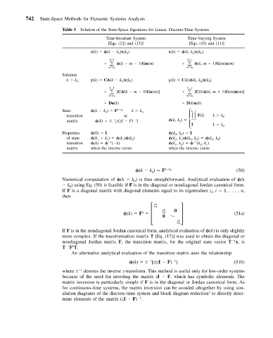
742 State-Space Methods for Dynamic Systems Analysis

Table 5 Solution of the State-Space Equations for Linear, Discrete-Time Systems
Time-Invariant System Time-Varying System
[Eqs. (12) and (13)] [Eqs. (10) and (11)]
x(k) (k k )x(k ) x(k) (k, k )x(k )
0 0 0 0
(k m 1)Gu(m) (k, m 1)G(m)u(m)
k 1
k 1
m k 0 m k 0
Solution
y(k) C (k k )x(k ) y(k) C(k) (k, k )x(k )
k k 0 0 0 0 0
[C (k m 1)Gu(m)] [C(k) (k, m 1)G(m)u(m)]
k 1
k 1
m k 0 m k 0
Du(k) D(k)u(k)
State (k k 0 ) F k k 0 k k 0
k 1
transition or
F(l) k k 0
1
1
matrix (k) L [z(zI F) ] (k, k ) l k k k 0
0
I
Properties (0) I (k 0 , k 0 ) I
of state (k 1 k 2 ) (k 1 ) (k 2 ) (k 2 , k 1 ) (k 1 , k 0 ) (k 2 , k 0 )
1
1
transition (k) ( k) (k 1 , k 2 ) (k 2 , k 1 )
matrix when the inverse exists when the inverse exists
(k k ) F k k 0 (50)
0
Numerical computation of (k k ) is thus straightforward. Analytical evaluation of (k
0
k ) using Eq. (50) is feasible if F is in the diagonal or nondiagonal Jordan canonical form.
0
If F is a diagonal matrix with diagonal elements equal to its eigenvalues z , i 1,..., n,
i
then
z k 1 z k 0
(k) F 0 2 (51a)
k
z k n
If F is in the nondiagonal Jordan canonical form, analytical evaluation of (k) is only slightly
more complex. If the transformation matrix T [Eq. (17)] was used to obtain the diagonal or
1
nondiagonal Jordan matrix F, the transition matrix, for the original state vector T x,is
1
k
T F T.
An alternative analytical evaluation of the transition matrix uses the relationship
1
(k) L [z(zI F) ] (51b)
1
1
where L denotes the inverse z-transform. This method is useful only for low-order systems
because of the need for inverting the matrix zI F, which has symbolic elements. The
matrix inversion is particularly simple if F is in the diagonal or Jordan canonical form. As
for continuous-time systems, the matrix inversion can be avoided altogether by using sim-
2
ulation diagrams of the discrete-time system and block diagram reduction to directly deter-
1
mine elements of the matrix (zI F) .