Page 763 - Mechanical Engineers' Handbook (Volume 2)

754 State-Space Methods for Dynamic Systems Analysis

1

3
–
–
1
0
2
2
H(s) 0 1 1 0
s 1 s 3
1 [1
–]
[0 1]
[0 –]
[1 0]
0
0
1
3
1
0 2 1 0 2 1
(75)
s 1 s 3
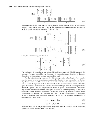
It should be noted that the number of vector products each coefficient matrix is factored into
is equal to the rank of the matrix. Then H(s) is written in a form that indicates the matrices
1
A, B, C clearly, by comparison with C(sI A) B:
s 1
1

H(s)
s 1 1 0 1 – 1 2
1010
1
0
1
0101 0 s 3 0 1 – 3 2
0
1
s 3

1010 s 1 s 1 0 1 0 – 2
1
1
2
1
0101 0 s 3 0 – 3 (76)
s 3 1 0
Thus, the corresponding realization is
1 1 0 1 – 1 2
1
2
0
A 0 3 B 0 – 3
C
1010 3 1 0 (77)
0101
The realization is controllable and observable and hence minimal. Modifications of this
procedure for cases where H(s) has elements with repeated poles are described by Brogan. 4
Extensions to discrete-time systems are straightforward.
An alternative two-step procedure for determining a minimal realization for a transfer
function matrix involves obtaining a nonminimal realization by any one method as the first
step. For example, one of the many realizations in Table 1 (Table 3 for discrete-time systems)
can be chosen to represent each of the elements of the transfer function matrix. The state-
space descriptions of the elements can then be combined to get the state-space equations for
the MIMO system. The resulting realization would, in general, be nonminimal. The second
step requires transformation of the state-space equations to the form given by Eq. (68) or an
equivalent one for discrete-time systems. Techniques for selecting the transformation matrix
9
1
are described by Kalman and Fortmann and Hitz. The minimal realization is then given
by the controllable and observable subsystem in Fig. 4. The resulting equations for a
continuous-time system are
˙ x Ax Bu (78)
21
m
22 m
y Cx Du (79)
12 m
m
where the subscript m indicates a minimal realization. Similar results for discrete-time sys-
7
4
tems are given by Brogan, Kuo, and Kalman. 9