Page 311 - PRINCIPLES OF QUANTUM MECHANICS as Applied to Chemistry and Chemical Physics

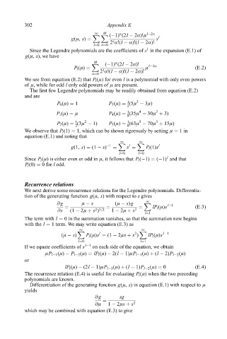
302 Appendix E
1 M á lÿ2á
X X (ÿ1) (2l ÿ 2á)!ì
g(ì, s) ˆ s l
l
2 á!(l ÿ á)!(l ÿ 2á)!
lˆ0 áˆ0
l
Since the Legendre polynomials are the coef®cients of s in the expansion (E.1) of
g(ì, s), we have
M á
X (ÿ1) (2l ÿ 2á)! lÿ2á
P l (ì) ˆ ì (E:2)
l
2 á!(l ÿ á)!(l ÿ 2á)!
áˆ0
We see from equation (E.2) that P l (ì) for even l is a polynomial with only even powers
of ì, while for odd l only odd powers of ì are present.
The ®rst few Legendre polynomials may be readily obtained from equation (E.2)
and are
3
1
P 0 (ì) ˆ 1 P 3 (ì) ˆ (5ì ÿ 3ì)
2
2
4
1
P 1 (ì) ˆ ì P 4 (ì) ˆ (35ì ÿ 30ì ‡ 3)
8
1
1
3
2
5
P 2 (ì) ˆ (3ì ÿ 1) P 5 (ì) ˆ (63ì ÿ 70ì ‡ 15ì)
2 8
We observe that P l (1) ˆ 1, which can be shown rigorously by setting ì ˆ 1in
equation (E.1) and noting that
1 1
X X
l
g(1, s) ˆ (1 ÿ s) ÿ1 ˆ s ˆ P l (1)s l
lˆ0 lˆ0
l
Since P l (ì) is either even or odd in ì, it follows that P l (ÿ1) ˆ (ÿ1) and that
P l (0) ˆ 0 for l odd.
Recurrence relations
We next derive some recurrence relations for the Legendre polynomials. Differentia-
tion of the generating function g(ì, s) with respect to s gives
1
@ g ì ÿ s (ì ÿ s)g X lÿ1
ˆ ˆ ˆ lP l (ì)s (E:3)
2 3=2
@s (1 ÿ 2ì ‡ s ) 1 ÿ 2ì ‡ s 2
lˆ1
The term with l ˆ 0 in the summation vanishes, so that the summation now begins
with the l ˆ 1 term. We may write equation (E.3) as
1 1
X X
2
l
(ì ÿ s) P l (ì)s ˆ (1 ÿ 2ìs ‡ s ) lP l (ì)s lÿ1
lˆ0 lˆ1
If we equate coef®cients of s lÿ1 on each side of the equation, we obtain
ìP lÿ1 (ì) ÿ P lÿ2 (ì) ˆ lP l (ì) ÿ 2(l ÿ 1)ìP lÿ1 (ì) ‡ (l ÿ 2)P lÿ2 (ì)
or
lP l (ì) ÿ (2l ÿ 1)ìP lÿ1 (ì) ‡ (l ÿ 1)P lÿ2 (ì) ˆ 0 (E:4)
The recurrence relation (E.4) is useful for evaluating P l (ì) when the two preceding
polynomials are known.
Differentiation of the generating function g(ì, s) in equation (E.1) with respect to ì
yields
@ g sg
ˆ
@ì 1 ÿ 2ìs ‡ s 2
which may be combined with equation (E.3) to give