Page 1013 - The Mechatronics Handbook

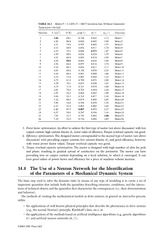
TABLE 34.3 Motor P = 5.5 kW, U = 380 V Solutions List, Without Generated
Parameters Limited
3
Number V [dm ] ϑ [K] cosϕ [-] η [-] m p [-] Directory
1 3.96 88.1 0.798 0.834 1.72 Motor1
2 4.20 86.9 0.818 0.843 1.90 Motor2
3 4.31 74.9 0.787 0.865 1.77 Motor3
4 4.32 88.8 0.836 0.817 1.78 Motor4
5 4.33 75.1 0.690 0.973 1.07 Motor5
6 4.50 89.0 0.836 0.834 1.79 Motor6
7 4.51 86.8 0.818 0.818 1.93 Motor7
8 4.54 90.0 0.884 0.812 1.98 Motor8
9 4.56 84.6 0.857 0.816 1.74 Motor9
10 4.58 86.5 0.836 0.817 1.77 Motor10
11 4.63 68.2 0.792 0.858 2.10 Motor11
12 4.69 88.4 0.862 0.808 1.80 Motor12
13 4.70 73.4 0.845 0.830 2.25 Motor13
14 4.73 61.0 0.799 0.871 1.90 Motor14
15 4.78 78.1 0.853 0.858 1.67 Motor15
16 4.78 71.0 0.767 0.870 1.80 Motor16
17 4.81 70.6 0.703 0.934 1.28 Motor17
18 4.97 54.5 0.804 0.883 1.90 Motor18
19 5.08 55.5 0.762 0.877 2.20 Motor19
20 5.12 88.2 0.879 0.806 2.05 Motor20
21 5.96 44.0 0.784 0.870 2.55 Motor21
22 6.35 42.4 0.803 0.882 2.69 Motor22
23 6.40 87.5 0.887 0.853 2.27 Motor23
24 6.57 59.0 0.747 0.956 1.16 Motor24
25 7.05 42.3 0.793 0.865 3.00 Motor25
26 7.39 52.9 0.714 0.986 1.03 Motor26

3. Power factor optimization. An effort to achieve the first type of motor (see above discussion) with low
copper content, high current density σ 1 , worse value of efficiency. Torque overload capacity was good.
4. Efficiency optimization. The designed motor corresponded to the second type of motor (see above
discussion) with prevailing copper content, low current density σ 1 , and good efficiency, however,
with worse power factor values. Torque overload capacity was good.
5. Torque overload capacity optimization. The motor is designed with high number of slots for pole
and phase, resulting in gradual spread of conductors on the perimeter. The motor can have
prevailing iron or copper content depending on a local solution, to which it converged. It can
have good values of power factor and efficiency for a price of machine volume increase.

34.4 The Use of a Neuron Network for the Identification
of the Parameters of a Mechanical Dynamic System

The basic step used to solve the dynamic tasks by means of any type of modeling is to create a set of
important quantities that include both the quantities describing structure, conditions, and the interac-
tions of technical objects and the quantities that characterize the consequences (i.e., their demonstration
and behavior).
The methods of creating the mathematical models in drive systems, in general an interactive process,
utilize
• the applications of well-known physical principles that describe the phenomena in drive systems

(e.g., the second Newton’s principle, Kirchhoff’s laws, etc.), or
• the applications of the methods based on artificial intelligence algorithms (e.g., genetic algorithms
[1] and artificial neuron networks [6, 7]).

©2002 CRC Press LLC