Page 885 - The Mechatronics Handbook

0066-frame-C29 Page 15 Wednesday, January 9, 2002 7:23 PM

5
x 10
1
Acceleration 0.5 0

-0.5
-1
0 0.1 0.2 0.3 0.4 0.5 0.6
Time (s)

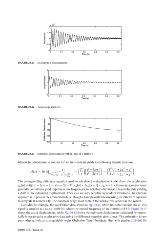
FIGURE 29.11 Acceleration measurement.

2 1
Displacement 0

-2 -1
0 0.1 0.2 0.3 0.4 0.5 0.6
Time (s)

FIGURE 29.12 Actual displacement.

0
Estimated Displacement -100
-50

-150
-200
0 0.1 0.2 0.3 0.4 0.5 0.6
Time (s)

FIGURE 29.13 Estimated displacement without use of a prefilter.

2
bilinear transformation to convert 1/s to the z-domain yields the following transfer function,
−1
2
1
Hz() = Hs()| 2 z−1) = --- =  T 2   z + 2z + 1   T 2   1 + 2z + z −2 
------------------------- =
--------------------------------
-----
------
(

−2
1
2
(
s=------------------ 2 2 z−1)  4  z – 2z +   4   −1
(
Tz +1) s s=------------------ 12z +– z
(
Tz +1)
The corresponding difference equation used to calculate the displacement y[•] from the acceleration
2
y dd [•] is 4(y[n] − 2y[n − 1] + y[n − 2]) = T (y dd [n] + 2y dd [n − 1] + y dd [n − 2]). However, accelerometers
generally do not have good response at low frequencies; in fact, they often insert a bias in the data yielding
a drift in the calculated displacement. They also are very sensitive to random vibrations. An alternate
approach is to process the acceleration data through a bandpass filter before using the difference equation
to integrate it numerically. The bandpass range must contain the natural frequencies in the system.
Consider, for example, the acceleration data shown in Fig. 29.11, which has some random noise. This
signal is sampled at a rate of 6400 Hz, where the natural frequency of the system is 50 Hz. Figure 29.12
shows the actual displacement, while Fig. 29.13 shows the estimated displacement calculated by numer-
ically integrating the acceleration data, using the difference equation given above. This estimation is very
poor. Alternatively, an analog eighth-order Chebyshev Type I bandpass filter with passband 25–500 Hz
©2002 CRC Press LLC