Page 886 - The Mechatronics Handbook

0066-frame-C29 Page 16 Wednesday, January 9, 2002 7:23 PM

2
Estimated Displacement 0 1

-2 -1
0 0.1 0.2 0.3 0.4 0.5 0.6
Time (s)
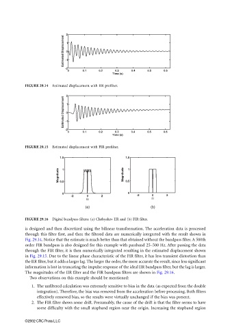
FIGURE 29.14 Estimated displacement with IIR prefilter.

2
Estimated Displacement 0 1

-2 -1
0 0.1 0.2 0.3 0.4 0.5 0.6
Time (s)
FIGURE 29.15 Estimated displacement with FIR prefilter.

1.5 1.5

Magnitude 0.5 1 Magnitude 0.5 1

0 0
-2 0 2 -2 0 2
Ω Ω
(a) (b)

FIGURE 29.16 Digital bandpass filters: (a) Chebyshev IIR and (b) FIR filter.

is designed and then discretized using the bilinear transformation. The acceleration data is processed
through this filter first, and then the filtered data are numerically integrated with the result shown in
Fig. 29.14. Notice that the estimate is much better than that obtained without the bandpass filter. A 500th
order FIR bandpass is also designed for this example with passband 25–500 Hz. After passing the data
through the FIR filter, it is then numerically integrated resulting in the estimated displacement shown
in Fig. 29.15. Due to the linear phase characteristic of the FIR filter, it has less transient distortion than
the IIR filter, but it adds a larger lag. The larger the order, the more accurate the result, since less significant
information is lost in truncating the impulse response of the ideal IIR bandpass filter, but the lag is larger.
The magnitudes of the IIR filter and the FIR bandpass filters are shown in Fig. 29.16.
Two observations on this example should be mentioned:
1. The unfiltered calculation was extremely sensitive to bias in the data (as expected from the double
integration). Therefore, the bias was removed from the acceleration before processing. Both filters
effectively removed bias, so the results were virtually unchanged if the bias was present.
2. The FIR filter shows some drift. Presumably, the cause of the drift is that the filter seems to have
some difficulty with the small stopband region near the origin. Increasing the stopband region

©2002 CRC Press LLC