Page 887 - The Mechatronics Handbook

0066-frame-C29 Page 17 Wednesday, January 9, 2002 7:23 PM

does reduce the drift. This can be done by decreasing the sample frequency or by increasing the
passband frequency. Both of these remedies decrease the drift but increase other errors in the
signal. Increasing the length of the filter decreases the drift error without introducing other errors.
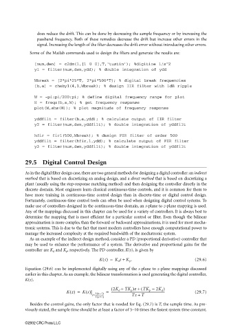
Some of the Matlab commands used to design the filters and generate the results are:

[num,den] = c2dm(1,[1 0 0],T,‘tustin’); %digitize 1/s^2
y1 = filter(num,den,ydd); % double integration of ydd

Wbreak = [2*pi*25*T, 2*pi*500*T}; % digital break frequencies
[b,a] = cheby1(4,1,Wbreak); % design IIR filter with 1dB ripple

W = -pi:pi/200:pi; % define digital frequency range for plot
H = freqz(b,a,W); % get frequency response
plot(W,abs(H)); % plot magnitude of frequency response

yddfilt = filter(b,a,ydd); % calculate output of IIR filter
y2 = filter(num,den,yddfilt); % double integration of yddfilt

hfir = fir1(500,Wbreak); % design FIR filter of order 500
yddfilt = filter(hfir,1,ydd); % calculate output of FIR filter
y3 = filter(num,den,yddfilt); % double integration of yddfilt

29.5 Digital Control Design

As in the digital filter design case, there are two general methods for designing a digital controller: an indirect
method that is based on discretizing an analog design, and a direct method that is based on discretizing a
plant (usually using the step-response matching method) and then designing the controller directly in the
discrete domain. Most engineers learn classical continuous-time controls, and it is common for them to
have more training in continuous-time control design than in discrete-time or digital control design.
Fortunately, continuous-time control tools can often be used when designing digital control systems. To
make use of controllers designed in the continuous-time domain, an s-plane to z-plane mapping is used.
Any of the mappings discussed in this chapter can be used for a variety of controllers. It is always best to
determine the mapping that is most efficient for a particular control or filter. Even though the bilinear
approximation is more complex than the forward or backward approximations, it is used for most mecha-
tronic systems. This is due to the fact that most modern controllers have enough computational power to
manage the increased complexity at the required bandwidth of the mechatronic system.
As an example of the indirect design method, consider a PD (proportional derivative) controller that
may be used to enhance the performance of a system. The derivative and proportional gains for the
controller are K d and K p , respectively. The PD controller, K(s), is given by
Ks() = K d s + K p . (29.6)

Equation (29.6) can be implemented digitally using any of the s-plane to z-plane mappings discussed
earlier in this chapter. As an example, the bilinear transformation is used generating the digital controller,
K(z).
( 2K d + TK p )z + ( TK p − 2K d )
Kz() = Ks()| 2 z−1) = ---------------------------------------------------------------------- (29.7)
(
s=------------------ Tz + T
(
Tz +1)
Besides the control gains, the only factor that is needed for Eq. (29.7) is T, the sample time. As pre-
viously stated, the sample time should be at least a factor of 5–10 times the fastest system time constant.

©2002 CRC Press LLC