Page 888 - The Mechatronics Handbook

0066-frame-C29 Page 18 Wednesday, January 9, 2002 7:23 PM

However, sampling times are often chosen to be several hundred times faster than the fastest system time
constant. An alternative strategy for a feedback system is to choose the sample rate to be at least 20 times
the desired closed loop bandwidth. Having sampling times that are substantially faster than the actual system
mitigates any differences between the controller as it is designed in the continuous domain and the imple-
mentation in the discrete domain. It should be noted that as the sampling frequency becomes higher, the
control gains become smaller. For example, in Eq. (29.7), as the sampling time becomes smaller, T becomes
smaller requiring better numerical resolution for the controller gains. If T becomes smaller than the
controller’s numerical gain resolution, it may be erroneously implemented at a value of 0 (zero) yielding
an incorrect control law.

Digital Control Example
Consider a high speed position motor with motor dynamics governed by the first-order equation

w s()
Gs() = -------------- = ------------------
K m
V in s() T m s + 1
where K m is the motor gain constant, T m is the motor time constant, ω(s) is the Laplace transform of the
motor velocity, and V in (s) is the Laplace transform of the motor input voltage. To determine the values
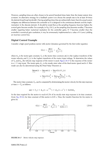
of T m and K m , the velocity step response of the motor is used. Figure 29.17 is the response of the motor
to a 1-V step input. The motor gain, K m , is the steady-state value of the final motor speed and is 5. This
result can also be determined using the Final Value Theorem as

lim w t() = lim sw s() = lim sG s()V in s()
t→∞ s→0 s→0
1
1
= lim sG s()-- = lim s-------------------- = K m
K m
1
s→0 s s→0 T m s + s
The motor time constant, T m , can be computed by determining the motor velocity for the step response
at time t = T m as follows:
−1
(
(
w t = T m ) = K m 1 e −t/T m ) = K m 1 e ) = 0.632K m
(
–
–
So the time required for the motor to reach 63.2% of its steady-state step response is its time constant.
From Fig. 29.18, the time constant of this motor is 0.05 s. Thus, the transfer function for the motor is
given by
w s() 5
Gs() = -------------- = ------------------ = --------------------- (29.8)
K m
V in s() T m s + 1 0.05s + 1

5 4
Motor Velocity (deg/s) 3 2

0 1
0 0.05 0.1 0.15 0.2 0.25 0.3 0.35
Time (s)

FIGURE 29.17 Motor velocity step response.

©2002 CRC Press LLC