Page 907 - The Mechatronics Handbook

0066_Frame_C30 Page 18 Thursday, January 10, 2002 4:43 PM

2
Computation of H Optimal Controller. The “mksys” command was used to pack the above two-port state
space into a tree vector data structure. The “h2lqg” command was then used to obtain the optimal
controller. Note that the generalized plant is 4th order (two for plant P, one for sensitivity weighting W 1 ,
one for control weighting W 2 ). The optimal controller:
191.0813 s + 40) s + 2) s + 0.526)
(
(
(
K opt = -------------------------------------------------------------------------------------------------- (30.92)
( s + 1.915) s + 0.01) s +( 2 84.15s + 2133)
(
is also 4th order—the order of the generalized plant G. The pole at s = −0.01 is an approximate integrator—a
consequence of the heavy weighting that W I places on the sensitivity at low frequencies.
Closed Loop Analysis. The resulting closed loop poles (two plant P = G 22 , four from controller K opt ) are
as follows:
s = – 1, 2.0786 ± j0.8302, 40, 40, 39.9216 (30.93)
–
–
–
–
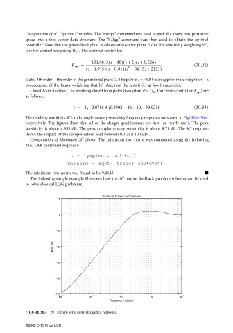
The resulting sensitivity, KS, and complementary sensitivity frequency responses are shown in Figs.30.4–30.6,
respectively. The figures show that all of the design specifications are met (or nearly met). The peak
sensitivity is about 4.855 dB. The peak complementary sensitivity is about 8.71 dB. The KS response
shows the impact of the compensators’ lead between 0.1 and 10 rad/s.
2
Computation of Minimum H Norm. The minimum two-norm was computed using the following
MATLAB command sequence:

lc = lyap(acl, bcl∗bcl)
minnorm = sqrt( trace( cc1∗c∗c’))

The minimum two-norm was found to be 9.0648.
2
The following simple example illustrates how the H output feedback problem solution can be used
to solve classical LQG problems.

Sensitivity Frequency Response
20

0

−20

Mag (dB) −40

−60

−80

−100 −1
10 −2 10 10 0 10 1 10 2
Frequency (rad/sec)
2
FIGURE 30.4 H Design sensitivity frequency response.

©2002 CRC Press LLC