Page 286 - Introduction to Statistical Pattern Recognition

268 Introduction to Statistical Pattern Recognition

1 n(n+2)
Jt?(V2p(X)}dX = 2"/2(27c)"/2 4 (6.66)

Accordingly, from (6.40)

*
I'= (6.67)

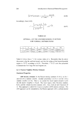
TABLE 6-1
OPTIMAL r OF THE UNIFORM KERNEL FUNCTION
FOR NORMAL DISTRIBUTIONS

Table 6-1 shows these r*'s for various values of n. Remember that the above
discussion is for the uniform kernel, and that the radius of the hyperellipsoidal
region is I.= according to (6.23). Therefore, I-*='s are also presented
to demonstrate how large the local regions are.

6.2 k Nearest Neighbor Density Estimate

Statistical Properties

RNN density estimate: In the Parzen density estimate of (6.1), we fix v
and let k be a random variable. Another possibility is to fix k and let v be a
random variable [12-161. That is, we extend the local region around X until
the kth nearest neighbor is found. The local region, then, becomes random,
L(X), and the volume becomes random, v(X). Also, both are now functions of
X. This approach is called the k nearest neighbor (kNN) density estimate. The
kNN approach can be interpreted as the Parzen approach with a uniform kernel