Page 52 - Introduction to Statistical Pattern Recognition

34 Introduction to Statistical Pattern Recognition

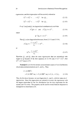
eigenvectors, and their eigenvalues will be reversely ordered as

h\’) > hi1) > . . . > ha’) for Q, , (2.1 12)

< hi2) < . . . < hi2) for Q2 . (2.113)

Proof Let Q and Q be diagonalized simultaneously such that
ATQA =I and ATQIA =A(’) , (2.114)

(2.115)

Then Q2 is also diagonalized because, from (2.1 11) and (2.1 14),

(2.1 16)

or

(2.1 17)

Therefore, Q, and Q2 share the same eigenvectors that are normalized with
respect to Q because of the first equation of (2.1 14) and, if hf” > A:”, then
hi2) < hj2) from (2.1 17).

Example 5: Let S be the mixture autocorrelation matrix of two distributions
whose autocorrelation matrices are S I and S 2. Then

s = E{XXT)
=PIE(XX*ICO~} +P2E(XXTI~2} =P IS1 +P,S;!. (2.118)

Thus, by the above theorem, we can diagonalize S I and S2 with the same set of
eigenvectors. Since the eigenvalues are ordered in reverse, the eigenvector with
the largest eigenvalue for the first distribution has the least eigenvalue for the
second, and vice versa. This property can be used to extract features important to
distinguish two distributions [8].