Page 101 - A First Course In Stochastic Models

TRANSIENT ANALYSIS 93

(n) (n) n
where the q and the p are the elements of the n-fold matrix products Q
ij ij
n
and P . State N can be reached from each starting state i = N under the Markov
(n) (n)
matrix P, since by assumption (b) p ≥ p > 0 for some n ≥ 1. Further, state
iN iN

N is absorbing under P. This implies that

(n)
lim p = 0 for all i, j = 1, . . . , N − 1,
n→∞ ij
n
as a special case of Lemma 3.2.3 below. Hence, by (3.2.6), lim n→∞ Q = 0. By
a standard result from linear algebra, it now follows that (3.2.5) has the unique
solution
µ = (I − Q) −1 e. (3.2.7)
This completes the proof that the linear equations (3.2.4) have a unique solution.

Example 3.1.1 (continued) The drunkard’s random walk
The drunkard moves over a square with the corner points (N, N), (−N, N),
(−N, −N) and (−N, N). It is interesting to see how the mean return time to
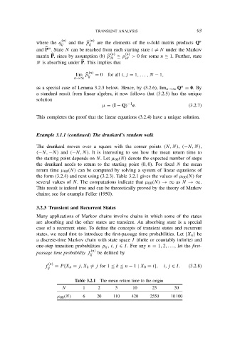
the starting point depends on N. Let µ 00 (N) denote the expected number of steps
the drunkard needs to return to the starting point (0, 0). For fixed N the mean
return time µ 00 (N) can be computed by solving a system of linear equations of
the form (3.2.4) and next using (3.2.3). Table 3.2.1 gives the values of µ 00 (N) for
several values of N. The computations indicate that µ 00 (N) → ∞ as N → ∞.
This result is indeed true and can be theoretically proved by the theory of Markov
chains; see for example Feller (1950).

3.2.3 Transient and Recurrent States
Many applications of Markov chains involve chains in which some of the states
are absorbing and the other states are transient. An absorbing state is a special
case of a recurrent state. To define the concepts of transient states and recurrent
states, we need first to introduce the first-passage time probabilities. Let {X n } be
a discrete-time Markov chain with state space I (finite or countably infinite) and
one-step transition probabilities p ij , i, j ∈ I. For any n = 1, 2, . . . , let the first-
(n)
passage time probability f be defined by
ij
(n)
f = P {X n = j, X k = j for 1 ≤ k ≤ n − 1 | X 0 = i}, i, j ∈ I. (3.2.8)
ij
Table 3.2.1 The mean return time to the origin
N 1 2 5 10 25 50
µ 00 (N) 6 20 110 420 2550 10 100