Page 114 - A First Course In Stochastic Models

106 DISCRETE-TIME MARKOV CHAINS

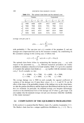
Table 3.3.1 The optimal claim limits and the minimal costs
Gamma Lognormal
2 2 2 2 2 2
c = 1 c = 4 c = 25 c = 1 c = 4 c = 25
D D D D D D
α ∗ 5908 6008 6280 6015 6065 6174
1
α ∗ 7800 7908 8236 7931 7983 8112
2
α ∗ 8595 8702 9007 8717 8769 8890
3
α ∗ 8345 8452 8757 8467 8519 8640
4
g ∗ 9058 7698 6030 9174 8318 7357
average cost per year is
4

g(α 1 , . . . , α 4 ) = c(j)π j
j=1
with probability 1. The one-year cost c(j) consists of the premium P j and any
damages not compensated that year by the insurance company. By conditioning on
the cumulative damage in the coming year, it follows that

α j

c(j) = P j + sg(s) ds + r j [1 − G(α j )].
0
The optimal claim limits follow by minimizing the function g(α 1 , . . . , α 4 ) with
respect to the parameters α 1 , . . . , α 4 . Efficient numerical procedures are widely
available to minimize a function of several variables. Table 3.3.1 gives for a number
∗
of examples the optimal claim limits α , . . . , α together with the minimal average
∗
1 4
∗
cost g . In all examples we take
P 1 = 10 000, P 2 = 7500, P 3 = 6000, P 4 = 5000,
r 1 = 1500, r 2 = 1000, r 3 = 750, r 4 = 500.
The average damage size is 5000 in each example; the squared coefficient of
variation of the damage size D takes three values: c 2 = 1, 4 and 25. To see the
D
effect of the shape of the probability density of the damage size on the claim limits,
we take the gamma distribution and the lognormal distribution both having the same
first two moments. In particular, the minimal average cost becomes increasingly
2
sensitive to the distributional form of the damage size D when c gets larger. Can
D
you explain why the minimal average cost per year decreases when the variability
of the claims increases?

3.4 COMPUTATION OF THE EQUILIBRIUM PROBABILITIES

In this section it is assumed that the Markov chain {X n } satisfies Assumption 3.3.1.
The Markov chain then has a unique equilibrium distribution {π j , j ∈ I}. The π j