Page 123 - A First Course In Stochastic Models

COMPUTATION OF THE EQUILIBRIUM PROBABILITIES 115

To analyse this queueing model, define the random variable X n by

X n = the number of messages in the buffer (excluding any message
in transmission) just prior to clock time t = n.

Then {X n , n = 0, 1, . . . } is a discrete-time Markov chain with the infinite state
space I = {0, 1, . . . }. The one-step transition probabilities are given by

λ j
−λ
p ij = e , 0 ≤ i < c and j = 0, 1, . . .
j!
λ j−i+c
−λ
p ij = e , i ≥ c and j = i − c, i − c + 1, . . . .
(j − i + c)!
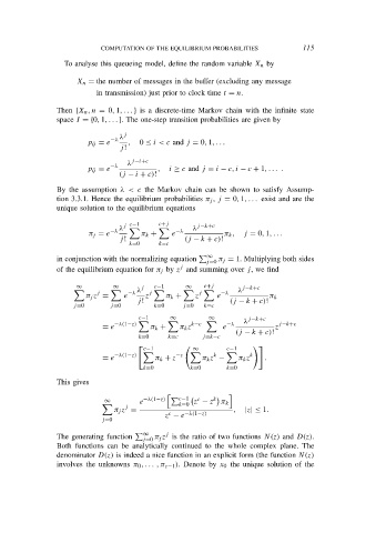
By the assumption λ < c the Markov chain can be shown to satisfy Assump-
tion 3.3.1. Hence the equilibrium probabilities π j , j = 0, 1, . . . exist and are the
unique solution to the equilibrium equations

j c−1 c+j j−k+c
λ λ
−λ −λ
π j = e π k + e π k , j = 0, 1, . . .
j! (j − k + c)!
k=0 k=c
∞
in conjunction with the normalizing equation
j=0 j = 1. Multiplying both sides
π
j
of the equilibrium equation for π j by z and summing over j, we find
∞ ∞ j c−1 ∞ c+j j−k+c
λ λ
j −λ j j −λ
π j z = e z π k + z e π k
j! (j − k + c)!
j=0 j=0 k=0 j=0 k=c
c−1 ∞ ∞ λ j−k+c
= e −λ(1−z) π k + π k z k−c e −λ z j−k+c
(j − k + c)!
k=0 k=c j=k−c
c−1 ∞ c−1

−λ(1−z) −c k k
= e π k + z π k z − π k z .
k=0 k=0 k=0
This gives

c
∞ e −λ(1−z)
c−1 z − z k
k=0 π k
j
π j z = c −λ(1−z) , |z| ≤ 1.
z − e
j=0

∞ j
The generating function j=0 j z is the ratio of two functions N(z) and D(z).
π
Both functions can be analytically continued to the whole complex plane. The
denominator D(z) is indeed a nice function in an explicit form (the function N(z)
involves the unknowns π 0 , . . . , π c−1 ). Denote by x 0 the unique solution of the