Page 292 - A First Course In Stochastic Models

286 SEMI-MARKOV DECISION PROCESSES

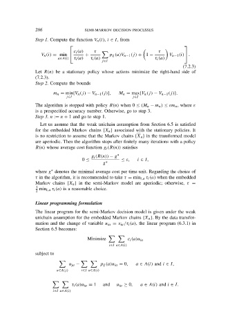
Step 1. Compute the function V n (i), i ∈ I, from
 
c i (a) τ τ
+ p ij (a)V n−1 (j) + 1 − V n−1 (i)  .
V n (i) = min 
a∈A(i) τ i (a) τ i (a) τ i (a)
j∈I
(7.2.3)
Let R(n) be a stationary policy whose actions minimize the right-hand side of
(7.2.3).
Step 2. Compute the bounds

m n = min{V n (j) − V n−1 (j)], M n = max{V n (j) − V n−1 (j)}.
j∈I j∈I
The algorithm is stopped with policy R(n) when 0 ≤ (M n − m n ) ≤ εm n , where ε
is a prespecified accuracy number. Otherwise, go to step 3.
Step 3. n := n + 1 and go to step 1.
Let us assume that the weak unichain assumption from Section 6.5 is satisfied
for the embedded Markov chains {X n } associated with the stationary policies. It
is no restriction to assume that the Markov chains {X n } in the transformed model
are aperiodic. Then the algorithm stops after finitely many iterations with a policy
R(n) whose average cost function g i (R(n)) satisfies
g i (R(n)) − g ∗
0 ≤ ≤ ε, i ∈ I,
g ∗
where g denotes the minimal average cost per time unit. Regarding the choice of
∗
τ in the algorithm, it is recommended to take τ = min i,a τ i (a) when the embedded
Markov chains {X n } in the semi-Markov model are aperiodic; otherwise, τ =
1
2 min i,a τ i (a) is a reasonable choice.
Linear programming formulation
The linear program for the semi-Markov decision model is given under the weak
unichain assumption for the embedded Markov chains {X n }. By the data transfor-
mation and the change of variable u ia = x ia /τ i (a), the linear program (6.3.1) in
Section 6.5 becomes:

Minimize c i (a)u ia
i∈I a∈A(i)
subject to

u ja − p ij (a)u ia = 0, a ∈ A(i) and i ∈ I,
a∈A(j) i∈I a∈A(i)

τ i (a)u ia = 1 and u ia ≥ 0, a ∈ A(i) and i ∈ I.
i∈I a∈A(i)