Page 405 - A First Course In Stochastic Models

400 ALGORITHMIC ANALYSIS OF QUEUEING MODELS

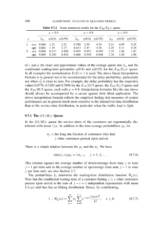
Table 9.7.1 Some numerical results for the E 10 /E 2 /c queue
ρ = 0.5 ρ = 0.8 ρ = 0.9
c L q η(0.8) η(0.95) L q η(0.8) η(0.95) L q η(0.8) η(0.95)
1 exa 0.066 1.21 2.21 0.780 2.59 4.78 2.21 4.99 9.25
app 0.082 1.19 2.17 0.813 2.57 4.76 2.25 5.14 9.25
5 exa 0.006 0.277 0.499 0.452 0.551 0.993 1.75 1.02 1.87
app 0.009 0.243 0.452 0.466 0.530 0.968 1.76 1.02 1.86

of c and ρ the exact and approximate values of the average queue size L q and the
conditional waiting-time percentiles η(0.8) and η(0.95) for the E 10 /E 2 /c queue.
In all examples the normalization E(S) = 1 is used. The above linear interpolation
formula is in general not to be recommended for the delay probability, particularly
2
not when c is close to zero. For example, the delay probability has the respective
S
values 0.0776, 0.3285 and 0.3896 for the E 10 /D/5 queue, the E 10 /E 2 /5 queue and
the E 10 /M/5 queue, each with ρ = 0.8. Interpolation formulas like the one above
should always be accompanied by a caveat against their blind application. The
above interpolation formula reflects the empirical finding that measures of system
performance are in general much more sensitive to the interarrival-time distribution
than to the service-time distribution, in particular when the traffic load is light.

9.7.1 The GI/M/c Queue
In the GI/M/c queue the service times of the customers are exponentially dis-
tributed with mean 1/µ. In addition to the time-average probabilities p j , let

π j = the long-run fraction of customers who find
j other customers present upon arrival.

There is a simple relation between the p j and the π j . We have

min(j, c)µp j = λπ j−1 , j = 1, 2, . . . . (9.7.6)

This relation equates the average number of downcrossings from state j to state
j − 1 per time unit to the average number of upcrossings from state j − 1 to state
j per time unit; see also Section 2.7.
The probabilities π j determine the waiting-time distribution function W q (x).
Note that the conditional waiting-time of a customer finding j ≥ c other customers
present upon arrival is the sum of j − c + 1 independent exponentials with mean
1/(cµ) and thus has an Erlang distribution. Hence, by conditioning,

∞ j−c k
−cµx (cµx)
1 − W q (x) = π j e , x ≥ 0. (9.7.7)
k!
j=c k=0