Page 411 - A First Course In Stochastic Models

406 ALGORITHMIC ANALYSIS OF QUEUEING MODELS

9.7.2 The GI/D/c Queue
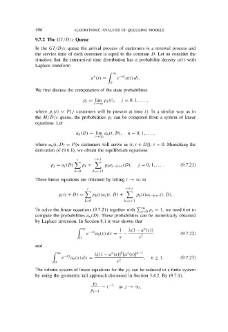
In the GI/D/c queue the arrival process of customers is a renewal process and
the service time of each customer is equal to the constant D. Let us consider the
situation that the interarrival-time distribution has a probability density a(t) with
Laplace transform

∞

∗ −st
a (s) = e a(t) dt.
0
We first discuss the computation of the state probabilities
p j = lim p j (t), j = 0, 1, . . . ,
t→∞
where p j (t) = P {j customers will be present at time t}. In a similar way as in
the M/D/c queue, the probabilities p j can be computed from a system of linear
equations. Let
a n (D) = lim a n (t, D), n = 0, 1, . . . ,
t→∞
where a n (t, D) = P {n customers will arrive in (t, t + D]}, t > 0. Mimicking the
derivation of (9.6.1), we obtain the equilibrium equations

c c+j

p j = a j (D) p k + p k a j−k+c (D), j = 0, 1, . . . . (9.7.21)
k=0 k=c+1
These linear equations are obtained by letting t → ∞ in

c c+j

p j (t + D) = p k (t)a j (t, D) + p k (t)a j−k+c (t, D).
k=0 k=c+1
To solve the linear equations (9.7.21) together with j=0 j = 1, we need first to
∞
p
compute the probabilities a n (D). These probabilities can be numerically obtained
by Laplace inversion. In Section 8.1 it was shown that
∗

∞ 1 λ(1 − a (s))
e −sx a 0 (x) dx = − 2 (9.7.22)
0 s s
and
∞ λ[(1 − a (s)] [a (s)]
2 n−1
∗
∗
e −sx a n (x) dx = 2 , n ≥ 1. (9.7.23)
0 s
The infinite system of linear equations for the p j can be reduced to a finite system
by using the geometric tail approach discussed in Section 3.4.2. By (9.7.1),
p j −1
∼ τ as j → ∞,
p j−1