Page 450 - A First Course In Stochastic Models

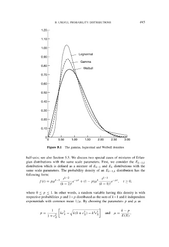
B. USEFUL PROBABILITY DISTRIBUTIONS 445

1.20

1.10

1.00
Lognormal
0.90
Gamma
0.80
Weibull
0.70

0.60

0.50

0.40

0.30

0.20

0.10

0
0 0.50 1.00 1.50 2.00 2.50 3.00
Figure B.1 The gamma, lognormal and Weibull densities

half-axis; see also Section 5.5. We discuss two special cases of mixtures of Erlan-
gian distributions with the same scale parameters. First, we consider the E k−1,k
distribution which is defined as a mixture of E k−1 and E k distributions with the
same scale parameters. The probability density of an E k−1,k distribution has the
following form:
t k−2 −µt k t k−1 −µt
k−1
f (t) = pµ e + (1 − p)µ e , t ≥ 0,
(k − 2)! (k − 1)!
where 0 ≤ p ≤ 1. In other words, a random variable having this density is with
respective probabilities p and 1−p distributed as the sum of k−1 and k independent
exponentials with common mean 1/µ. By choosing the parameters p and µ as

1 2 k − p
2
2 2
p = kc − k(1 + c ) − k c X and µ = ,
X
X
1 + c 2 E(X)
X