Page 46 - A First Course In Stochastic Models

RENEWAL THEORY 37

will be formulated in Section 8.2. For the moment it is sufficient to assume that
the interoccurrence times have a positive density on some interval. Further it is
2
assumed that µ 2 = E(X ) is finite. Then it will be shown in Theorem 8.2.3 that
1
t µ 2

lim M(t) − = 2 − 1. (2.1.6)
t→∞ µ 1 2µ
1
The approximation
t µ 2
M(t) ≈ + 2 − 1 for t large
µ 1 2µ
1
is practically useful for already moderate values of t provided that the squared
coefficient of variation of the interoccurrence times is not too large and not too
close to zero.

2.1.2 The Excess Variable
In many practical probability problems an important quantity is the random variable
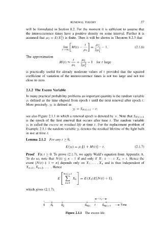
γ t defined as the time elapsed from epoch t until the next renewal after epoch t.
More precisely, γ t is defined as
γ t = S N(t)+1 − t;

see also Figure 2.1.1 in which a renewal epoch is denoted by ×. Note that S N(t)+1
is the epoch of the first renewal that occurs after time t. The random variable
γ t is called the excess or residual life at time t. For the replacement problem of
Example 2.1.1 the random variable γ t denotes the residual lifetime of the light bulb
in use at time t.

Lemma 2.1.2 For any t ≥ 0,
E(γ t ) = µ 1 [1 + M(t)] − t. (2.1.7)

Proof Fix t ≥ 0. To prove (2.1.7), we apply Wald’s equation from Appendix A.
To do so, note that N(t) ≤ n − 1 if and only if X 1 + · · · + X n > t. Hence the
event {N(t) + 1 = n} depends only on X 1 , . . . , X n and is thus independent of
X n+1 , X n+2 , . . . . Hence

 
N(t)+1

E  X k  = E(X 1 )E[N(t) + 1],
k=1
which gives (2.1.7).

g
t
0 S 1 S 2 S N(t) t S N(t) + 1 Time
Figure 2.1.1 The excess life