Page 460 - A First Course In Stochastic Models

D. THE DISCRETE FAST FOURIER TRANSFORM 455

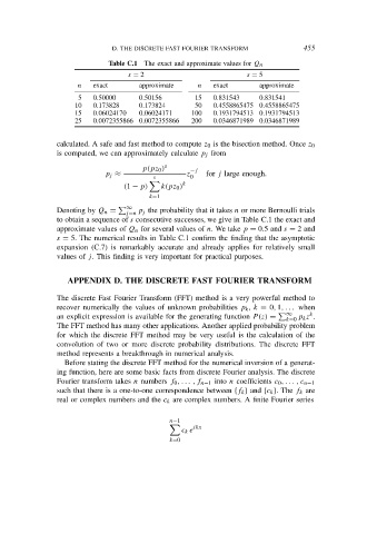
Table C.1 The exact and approximate values for Q n
s = 2 s = 5
n exact approximate n exact approximate
5 0.50000 0.50156 15 0.831543 0.831541
10 0.173828 0.173824 50 0.4558865475 0.4558865475
15 0.06024170 0.06024171 100 0.1931794513 0.1931794513
25 0.0072355866 0.0072355866 200 0.0346871989 0.0346871989

calculated. A safe and fast method to compute z 0 is the bisection method. Once z 0
is computed, we can approximately calculate p j from

p(pz 0 ) s −j
p j ≈ z for j large enough.
s 0
k
(1 − p) k(pz 0 )
k=1
∞

Denoting by Q n = p j the probability that it takes n or more Bernoulli trials
j=n
to obtain a sequence of s consecutive successes, we give in Table C.1 the exact and
approximate values of Q n for several values of n. We take p = 0.5 and s = 2 and
s = 5. The numerical results in Table C.1 confirm the finding that the asymptotic
expansion (C.7) is remarkably accurate and already applies for relatively small
values of j. This finding is very important for practical purposes.

APPENDIX D. THE DISCRETE FAST FOURIER TRANSFORM

The discrete Fast Fourier Transform (FFT) method is a very powerful method to
recover numerically the values of unknown probabilities p k , k = 0, 1, . . . when
∞

k
an explicit expression is available for the generating function P (z) = p k z .
k=0
The FFT method has many other applications. Another applied probability problem
for which the discrete FFT method may be very useful is the calculation of the
convolution of two or more discrete probability distributions. The discrete FFT
method represents a breakthrough in numerical analysis.
Before stating the discrete FFT method for the numerical inversion of a generat-
ing function, here are some basic facts from discrete Fourier analysis. The discrete
Fourier transform takes n numbers f 0 , . . . , f n−1 into n coefficients c 0 , . . . , c n−1
such that there is a one-to-one correspondence between {f k } and {c k }. The f k are
real or complex numbers and the c k are complex numbers. A finite Fourier series

n−1
ikx
c k e
k=0