Page 94 - A Practical Companion to Reservoir Stimulation

EVALUATION OF TREATMENTS AND POSTFRACTURE PERFORMANCE

EXAMPLE F-4
(1)( 100)(3000)
Prediction of the Beginning 4= = 9660 STB/d. (F-13)
and End of Bilinear Flow (141.2)(0.2)( 1.1)( I)
The end of bilinear flow is at = 1.5 x and therefore
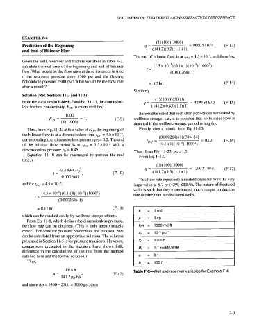
Given the well, reservoir and fracture variables in Table F-2,
calculate the real time of the beginning and end of bilinear (1.5 x ~o-~)(o.i)( 1)(10-~)( 1000~)
flow. What would be the flow rates at these instances in time t= (0.000264) ( 1 )
if the reservoir pressure were 5300 psi and the flowing
bottomhole pressure 2300 psi? What would be the flow rate = 5.7 hr. (F- 1 4)
after a month?
Similarly,
Solution (Ref. Sections 11-3 and 11-5)
From the variables in Table F-2 and Eq. 1 1- 1 1, the dimension- 4= (I)( 1000)(3000) = 4290STB/d. (F-15)
less fracture conductivity, F&, is calculated first. ' (141.2)(0.45)( 1.1)( I)
It should be noted that such short periods can be masked by
(F-9) wellbore storage; i.e., it is possible that no bilinear flow is
detected if the wellbore storage period is lengthy.
Thus, from Fig. 1 1-23 at this value of F&, the beginning of Finally, after a month, from Eq. 1 1 - 10,
the bilinear flow is at a dimensionless time tD.rj= 4.5 x lo-', (0.000264) ( 1) (30 x 24)
corresponding to a dimensionless pressure pD = 0.2. The end 'Dxf = = 0.19. (F-16)
of the bilinear flow period is at tD,f = 1.5~ with a (0.1 ) ( 1 ) ( 10-5) ( 10002)
dimensionless pressure pD = 0.45. Then, from Fig. 11-23, pD = 1.5.
Equation 11-10 can be rearranged to provide the real From Eq. F- 12,
time, t.
(1)( 100)(3000)
lDsJ qp c, x/ 4= = 1290STB/d. (F-17)
t= (F-10) (141.2)( 1.5)( 1.1)( 1)
0.000264k '
This flow rate represents a marked decrease from the very
and for tD,/ = 4.5 x large value at 5.7 hr (4290 STB/d). The nature of fractured
wells is such that they experience a much steeper production
(4.5 x 10-~)(0.1)( 1)(10-~)( 1000~) rate decline than nonfractured wells.
t=
(0.000264) ( 1 )
= 0.17 hr, (F-11) -p
which can be masked easily by wellbore storage effects.
From Eq. 1 1-8, which defines the dimensionless pressure,
the flow rate can be obtained. (This is only approximately k,w = 1000 md-ft
correct. For constant pressure production, the transient rate 4
I ct
= 10-5 psi-'
can be calculated from an appropriate solution. The solution
presented in Section I 1-5 is for pressure transients. However,
comparisons presented in the literature have shown little
difference in the calculations of the rate from the method
outlined here and the formal solution.)
Thus, = l00ft

khAp Table F-2-Well and reservoir variables for Example F-4.
4= (F-12)
14 1 .2pD Bp '
and since Ap = 5300 - 2300 = 3000 psi, then

F-3