Page 424 - A Course in Linear Algebra with Applications

408 Chapter Ten: Linear Programming

can be run. There is no loss in assuming that B > 0 since we
can, if necessary, multiply a constraint by —1.
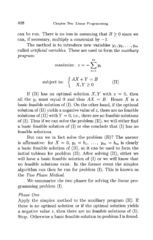
The method is to introduce new variables yi,V2,- • • ,y m
called artificial variables. These are used to form the auxiliary
program:

-J>*
maximize: z

subject to: <^ X Y >0 ^ '

If (II) has an optimal solution X, Y with z = 0, then
all the yi must equal 0 and thus AX = B. Hence X is a
basic feasible solution of (I). On the other hand, if the optimal
solution of (II) yields a negative value of 2, there are no feasible
solutions of (II) with Y = 0, i.e., there are no feasible solutions
of (I). Thus if we can solve the problem (II), we will either find
a basic feasible solution of (I) or else conclude that (I) has no
feasible solutions.
But can we in fact solve the problem (II)? The answer
is affirmative: for X = 0, y\ = b\, ..., y m = b m is clearly
a basic feasible solution of (II), so it can be used to form the
initial tableau for problem (II). After solving (II), either we
will have a basic feasible solution of (I) or we will know that
no feasible solutions exist. In the former event the simplex
algorithm can then be run for problem (I). This is known as
the Two Phase Method.
We summarize the two phases for solving the linear pro-
gramming problem (I).

Phase One
Apply the simplex method to the auxiliary program (II). If
there is no optimal solution or if the optimal solution yields
a negative value z, then there are no feasible solutions of (I).
Stop. Otherwise a basic feasible solution to problem I is found.