Page 68 - A Course in Linear Algebra with Applications

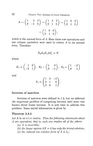
52 Chapter Two: Systems of Linear Equations

A^l 1 2 2 \ A 2 2 \ / I 0 2~
0 - 1 Oj \0 1 Oj \0 1 0

1 0 0
0 1 0

which is the normal form of A. Here three row operations and
one column operation were used to reduce A to its normal
form. Therefore

E 3E 2E 1AF 1 = N

where

* = | J ? ) . * = f j ?),*3=' 1 ^
-2 \) ' ^ V0 - 1 ) ' •* I 0 1

and

Inverses of matrices

Inverses of matrices were defined in 1.2, but we deferred
the important problem of computing inverses until more was
known about linear systems. It is now time to address this
problem. Some initial information is given by

Theorem 2.3.5
Let A be annxn matrix. Then the following statements about
A are equivalent, that is, each one implies all of the others.
(a) A is invertible;
(b) the linear system AX = 0 has only the trivial solution;
(c) the reduced row echelon form of A is I n;