Page 261 - Adaptive Identification and Control of Uncertain Systems with Nonsmooth Dynamics

262 Adaptive Identification and Control of Uncertain Systems with Non-smooth Dynamics

the following property

σ(a,b,c) = max(a, min(b,c)) (17.14)

It has been proven in [10] that any one-dimension piecewise linear function
(e.g., backlash) can be represented by (17.13).
In addition, when choosing the number of subintervals s, a trade-off
between the accuracy of identification and the calculation burden should
be considered. In general, a larger s will increase the calculation burden,
while the accuracy of identification can be improved. On the contrary, the
calculation burden is decreased with a small s, but the modeling accuracy
may be degraded. For the backlash non-linearity discussed in this chapter,
the value of s can be appropriately chosen as a constant between 10 to 15.
Note that σ(·) in DPPR (17.13) is a piecewise linear function. More-
over, the input of (17.13) is the realistic control u, and the unknown
parameters p j ,j = 0,··· ,s in (17.13) are linearly presented. Hence, we can
combine (17.13)togetherwithsystem(17.12), such that the unknown pa-
rameters p j ,α j ,β j can be estimated simultaneously by using the collected
sampling data u(k),y 0 (k). For this purpose, by substituting (17.13)into
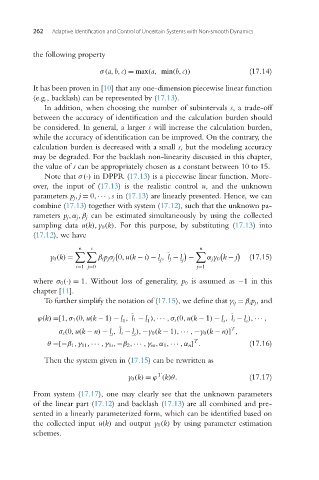
(17.12), we have

n s n

y 0 (k) = β ip j σ j 0,u(k − i) − l , l j − l − α jy 0 k − j (17.15)
j j
i=1 j=0 j=1
where σ 0 (·) = 1. Without loss of generality, p 0 is assumed as −1in this
chapter [11].
To further simplify the notation of (17.15), we define that γ ij = β ip j ,and

ϕ(k) =[1,σ 1 (0,u(k − 1) − l , l 1 − l ),··· ,σ s (0,u(k − 1) − l , l s − l ),··· ,
s
1
1
s
T
σ s (0,u(k − n) − l , l s − l ),−y 0 (k − 1),··· ,−y 0 (k − n)] ,
s s
T
θ =[−β 1 ,γ 11 ,··· ,γ 1s ,−β 2 ,··· ,γ ns ,α 1 ,··· ,α n ] . (17.16)
Then the system given in (17.15) can be rewritten as
T
y 0 (k) = ϕ (k)θ. (17.17)
From system (17.17), one may clearly see that the unknown parameters
of the linear part (17.12)and backlash (17.13) are all combined and pre-
sented in a linearly parameterized form, which can be identified based on
the collected input u(k) and output y 0 (k) by using parameter estimation
schemes.