Page 87 - Adaptive Identification and Control of Uncertain Systems with Nonsmooth Dynamics

RISE Based Asymptotic PPC of Servo Systems With Continuously Differentiable Friction Model 79

we will design a control such that the tracking control error e 1 (t) is not
only retained within the PPF bound (5.5) in the transient stage, but also
converges to zero in the steady-state. Thus, based on the property of the
error function (5.6)and (5.9), the transformed error z 1 must be controlled
to converge to zero even in the presence of uncertainties and disturbances.
For this purpose, we will present a new control strategy by extending the
RISE method [11].

5.3.1 Derivation of Filtered Tracking Error

To facility controller design, we define state variables x =[x 1 ,x 2 ]=[q, ˙q]
and x d = q d , and the tracking error e 1 = x 1 − x d , then the following filter
errors are obtained as
z 2 =˙z 1 + k 1z 1
(5.10)
r =˙z 2 + k 2z 2
where k 1 and k 2 are positive constants selected by the designers. It has been
shown in [11] that the auxiliary filter error r is not available for the control
design because ˙z 2 is not measurable. However, it can provide an alternative
method to analyze the system stability and robustness.
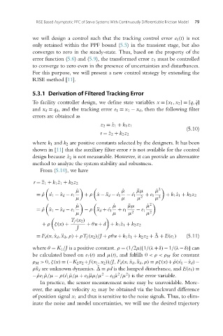
From (5.10), we have

r =¨z 1 + k 1 ˙z 1 + k 2z 2
2
˙ μ ˙ μ ¨ μμ ˙ μ
ρ
˙
=˙ x 1 −¨x d − e 1 + ρ ˙ x −¨x d −¨e 1 −¨ e 1 2 + e 1 2 + k 1 ˙z 1 + k 2z 2
μ μ μ μ
2
˙ μ ˙ μ ¨ μμ ˙ μ
ρ
=˙ ˙x 1 −¨x d − e 1 − ρ ¨ x d +˙e 1 + e 1 2 − e 1 2
μ μ μ μ

T f (x 2 )
+ ρ ζ(x) + + θu + d + k 1 ˙z 1 + k 2z 2
J
= F d (x, ˙x d , ¨x d ,ρ) + ρT f (x 2 )/J + ρθu + k 1 ˙z 1 + k 2z 2 + + E(e 1 ) (5.11)
˜
where θ = K 1 /J is a positive constant. ρ = (1/2μ)[1/(λ+δ)−1/(λ−δ)] can
be calculated based on e 1 (t) and μ(t), and fulfills 0 <ρ <ρ M for constant
x
ρ M > 0, ζ(x) = (−K 2x 2 +f (x 1 ,x 2 ))/J, F d (x, ˙x d , ¨x d ,ρ) = ρζ(x)+˙ρ( ˙ 1 −¨x d )−
˜
ρ ¨ x d are unknown dynamics. = ρd is the lumped disturbance, and E(e 1 ) =
2
2
2
−¨e 1 ˙μ/μ − ρ( ˙e 1 ˙μ/μ + e 1 ¨μμ/μ − e 1 ˙μ /μ ) is the error variable.
ρ
In practice, the sensor measurement noise may be unavoidable. More-
over, the angular velocity x 2 may be obtained via the backward difference
of position signal x 1 and thus is sensitive to the noise signals. Thus, to elim-
inate the noise and model uncertainties, we will use the desired trajectory