Page 812 - Advanced_Engineering_Mathematics o'neil

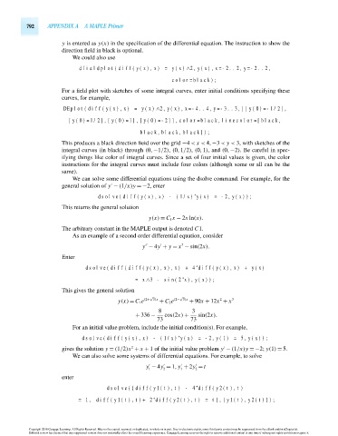
792 APPENDIX A A MAPLE Primer

y is entered as y(x) in the specification of the differential equation. The instruction to show the
direction field in black is optional.
We could also use

dfieldplot(diff(y(x),x) = y(x)∧2,y(x),x=-2..2,y=-2..2,
color=black);
For a field plot with sketches of some integral curves, enter initial conditions specifying these
curves, for example,
DEplot(diff(y(x),x) = y(x)∧2,y(x),x=-4..4,y=-3..3,[[y(0)=-1/2],
[y(0)=1/2],[y(0)=1],[y(0)=-2]],color=black,linecolor=[black,

black,black,black]);
This produces a black direction fieid over the grid −4 < x < 4,−3 < y < 3, with sketches of the
integral curves (in black) through (0,−1/2), (0,1/2), (0,1), and (0,−2). Be careful in spec-
ifying things like color of integral curves. Since a set of four initial values is given, the color
instructions for the integral curves must include four colors (although some or all can be the
same).
We can solve some differential equations using the dsolve command. For example, for the

general solution of y − (1/x)y =−2, enter
∗
dsolve(diff(y(x),x) - (1/x) y(x) = -2,y(x));
This returns the general solution

y(x) = C 1 x − 2x ln(x).
The arbitrary constant in the MAPLE output is denoted C1.
As an example of a second order differential equation, consider
3
y − 4y + y = x − sin(2x).

Enter
∗
dsolve(diff(diff(y(x),x),x) + 4 diff(y(x),x) + y(x)
=x∧3 - sin(2 x),y(x));
∗
This gives the general solution
√ √
2
y(x) =C 1 e (2+ 3)x + C 2 e (2− 3)x + 90x + 12x + x 3
8 3
+ 336 − cos(2x) + sin(2x).
73 73
For an initial value problem, include the initial condition(s). For example,
∗
dsolve(diff(y(x),x) - (1/x) y(x) = -2,y(1) = 5,y(x));
2
gives the solution y = (1/2)x + x + 1 of the initial value problem y − (1/x)y =−2; y(1) = 5.

We can also solve some systems of differential equations. For example, to solve

y − 4y = 1, y + 2y = t

1 2 1 2
enter
∗
dsolve({diff(y1(t),t) - 4 diff(y2(t),t)
∗
= 1, diff(y1(t),t)+ 2 diff(y2(t),t) = t},{y1(t),y2(t)});

Copyright 2010 Cengage Learning. All Rights Reserved. May not be copied, scanned, or duplicated, in whole or in part. Due to electronic rights, some third party content may be suppressed from the eBook and/or eChapter(s).
Editorial review has deemed that any suppressed content does not materially affect the overall learning experience. Cengage Learning reserves the right to remove additional content at any time if subsequent rights restrictions require it.

October 14, 2010 15:43 THM/NEIL Page-792 27410_24_appA_p789-800