Page 255 - Advanced engineering mathematics

7.8 Least Squares Vectors and Data Fitting 235

Finally,
⎛ ⎞
3

−112 9
t
A B = ⎝ −2 ⎠ = .
−242 0
7
The auxiliary lsv system is

6 10 9
X = .
10 24 0
This has a unique solution, which is the unique least squares vector for the system:
−1
6 10 9 12/22 −5/22 9 108/22
∗ .
X = = =
10 24 0 −5/22 3/22 0 −45/22
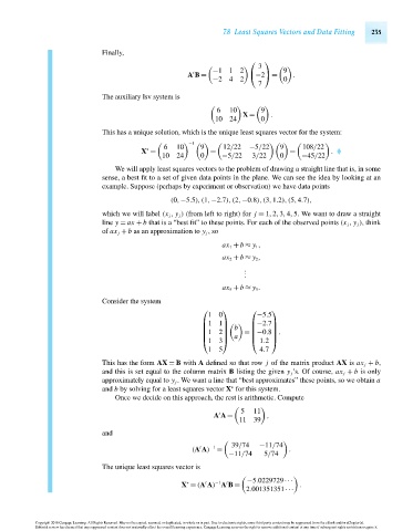
We will apply least squares vectors to the problem of drawing a straight line that is, in some
sense, a best fit to a set of given data points in the plane. We can see the idea by looking at an
example. Suppose (perhaps by experiment or observation) we have data points

(0,−5.5),(1,−2.7),(2,−0.8),(3,1.2),(5,4.7),
which we will label (x j , y j ) (from left to right) for j = 1,2,3,4,5. We want to draw a straight
line y = ax + b that is a “best fit” to these points. For each of the observed points (x j , y j ), think
of ax j + b as an approximation to y j ,so
ax 1 + b ≈ y 1 ,
ax 2 + b ≈ y 2 ,
.
.
.
ax 5 + b ≈ y 5 .

Consider the system
⎛ ⎞ ⎛ ⎞
10 −5.5
−2.7
11
⎜ ⎟ ⎜ ⎟
⎜ ⎟ b ⎜ ⎟
⎟
⎜
⎜ 12 ⎟ = −0.8 .
⎜ ⎟ a ⎜ ⎟
⎝ 13 ⎠ ⎝ 1.2 ⎠
15 4.7
This has the form AX = B with A defined so that row j of the matrix product AX is ax j + b,
and this is set equal to the column matrix B listing the given y j ’s. Of course, ax j + b is only
approximately equal to y j . We want a line that “best approximates” these points, so we obtain a
∗
and b by solving for a least squares vector X for this system.
Once we decide on this approach, the rest is arithmetic. Compute

5 11
t
A A = ,
11 39
and

39/74 −11/74
t −1
(A A) = .
−11/74 5/74
The unique least squares vector is

∗ t −1 t −5.0229729···
X = (A A) A B = .
2.001351351···

Copyright 2010 Cengage Learning. All Rights Reserved. May not be copied, scanned, or duplicated, in whole or in part. Due to electronic rights, some third party content may be suppressed from the eBook and/or eChapter(s).
Editorial review has deemed that any suppressed content does not materially affect the overall learning experience. Cengage Learning reserves the right to remove additional content at any time if subsequent rights restrictions require it.

October 14, 2010 14:23 THM/NEIL Page-235 27410_07_ch07_p187-246