Page 521 - Advanced engineering mathematics

14.7 DFT Approximation of the Fourier Transform 501

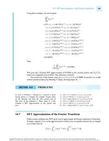
Using these numbers, we can compute
127
πik/2
V k e
k=0
=127 + (−1 + 40.735i)e πi/2 + (−1 + 20.355i)e πi
+ (−1 + 13.557i)e 3πi/2 + (−1 + 10.153i)e 2πi
+ (−1 + 8.1078i)e 5πi/2 + (−1 + 6.7415i)e 3πi
+ (−1 + 5.7631i)e 7πi/2 + (−1 + 5.0273i)e 4πi
+ (−1 + 4.4532i)e 9πi/2 + (−1 + 3.9922i)e 5πi

+ (−1 − 3.9922i)e 118πi/2 + (−1 − 4.4532i)e 1119πi/2
+ (−1 − 5.0273i)e 120πi/2 + (−1 − 5.7631i)e 121π/2
+ (−1 − 6.7415i)e 122πi/2 + (−1 − 8.1078i)e 123πi/2
+ (−1 − 10.153i)e 124πi/2 + (−1 − 13.557i)e 125πi/2
+ (−1 − 20.355i)e 126πi/2 + (−1 − 30.735i)e 127πi/2
=61.04832.

Then
127
1 πijk/64
V k e = 0.47694.
128
k=0
This gives the 128 point DFT approximation of 0.47694 to the sampled partial sum S 10 (1/2),
which was computed to be 0.45847. The difference is 0.0185.
The actual sum of the Fourier series at t = 1/2is f (1/2) = 0.50000. In practice we would
achieve greater accuracy by choosing N larger, allowing larger M.

SECTION 14.6 PROBLEMS

In each of Problems 1 through 6, a function is given 1. f (t) = 1 + t for 0 ≤ t < 2, p = 2, t 0 = 1/8
2
having period p. Compute the complex Fourier series 2. f (t) = t for 0 ≤ t < 1, p = 1, t 0 = 1/2
of the function and then the 10th partial sum of 3. f (t) = cos(t) for 0 ≤ t < 2, p = 2, t 0 = 1/8
this series at the indicated t 0 . Then, using N = 128, 4. f (t) = e −t for 0 ≤ t < 4, p = 4, t 0 = 1/4
3
compute a DFT approximation to this partial sum 5. f (t) = t for 0 ≤ t < 1, p = 1, t 0 = 1/4
at t 0 . 6. f (t) = t sin(t) for 0 ≤ t < 4, p = 4, t 0 = 1/8.

14.7 DFT Approximation of the Fourier Transform

Under certain conditions the DFT can be used to approximate the Fourier transform of a function.
ˆ
To begin, suppose f (ω) can be approximated to within some acceptable tolerance by an integral
over a finite interval
∞
2π L
ˆ
f (ω) = f (ξ)e −iωξ dξ ≈ f (ξ)e −iωξ dξ.
−∞ 0

Copyright 2010 Cengage Learning. All Rights Reserved. May not be copied, scanned, or duplicated, in whole or in part. Due to electronic rights, some third party content may be suppressed from the eBook and/or eChapter(s).
Editorial review has deemed that any suppressed content does not materially affect the overall learning experience. Cengage Learning reserves the right to remove additional content at any time if subsequent rights restrictions require it.

October 14, 2010 16:43 THM/NEIL Page-501 27410_14_ch14_p465-504