Page 64 - Advanced engineering mathematics

44 CHAPTER 2 Linear Second-Order Equations

and then once again to get
3
y(x) = 2x + cx + k
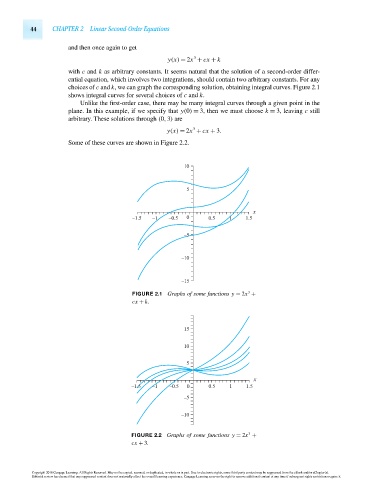
with c and k as arbitrary constants. It seems natural that the solution of a second-order differ-
ential equation, which involves two integrations, should contain two arbitrary constants. For any
choices of c and k, we can graph the corresponding solution, obtaining integral curves. Figure 2.1
shows integral curves for several choices of c and k.
Unlike the first-order case, there may be many integral curves through a given point in the
plane. In this example, if we specify that y(0) = 3, then we must choose k = 3, leaving c still
arbitrary. These solutions through (0,3) are
3
y(x) = 2x + cx + 3.
Some of these curves are shown in Figure 2.2.

10

5

x
–1.5 –1 –0.5 0 0.5 1 1.5

–5

–10

–15
3
FIGURE 2.1 Graphs of some functions y = 2x +
cx + k.

15

10

5

x
–1.5 –1 –0.5 0 0.5 1 1.5
–5

–10

3
FIGURE 2.2 Graphs of some functions y = 2x +
cx + 3.

Copyright 2010 Cengage Learning. All Rights Reserved. May not be copied, scanned, or duplicated, in whole or in part. Due to electronic rights, some third party content may be suppressed from the eBook and/or eChapter(s).
Editorial review has deemed that any suppressed content does not materially affect the overall learning experience. Cengage Learning reserves the right to remove additional content at any time if subsequent rights restrictions require it.

October 14, 2010 14:12 THM/NEIL Page-44 27410_02_ch02_p43-76