Page 158 - Aerodynamics for Engineering Students

Potential flow 141

Using Eqns (3.63) and (3.65) and Eqns (3.64) and (3.66) it can be seen that for a
point source at the origin placed in a uniform flow - U along the z axis
Q
+=-URCOS~-- (3.67a)
41rR
$=--UR2sin Z p--cos'p (3.67b)
Q
1
2 4Ir
The flow field represented by Eqns (3.67) corresponds to the potential flow around
a semi-finite body of revolution - very much like its two-dimensional counterpart
described in Section 3.3.5. In a similar way to the procedure described in Section 3.3.5
it can be shown that the stagnation point occurs at the point (-a, 0) where

(3.68)

and that the streamlines passing through this stagnation point define a body of
revolution given by

R~ = 2a2 ( 1 + cos cp) / sin2 'p (3.69)
The derivation of Eqns (3.68) and (3.69) are left as an exercise (see Ex. 19) for the
reader.
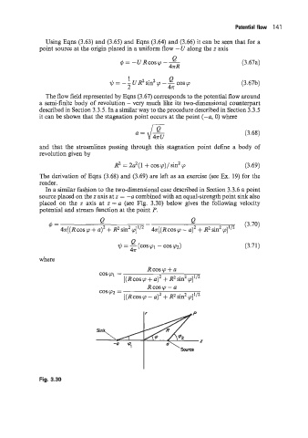
In a similar fashion to the two-dimensional case described in Section 3.3.6 a point
source placed on the z axis at z = -a combined with an equal-strength point sink also
placed on the z axis at z = a (see Fig. 3.30) below gives the following velocity
potential and stream function at the point P.
Q
+= Q (3.70)
4.rr[(Rcos 'p + a)' + R2 sin2 cp]'/2 - 41r[(Rcos cp - a)' + R2 sin2 cp]'/'

II, = Q (cos cp1 - cos 92) (3.71)

where
Rcos'p+a
COScpl =
+
[(Rcos'~+u)~ ~~sin~'p]'/~

Fig. 3.30