Page 140 - Algorithm Collections for Digital Signal Processing Applications using MATLAB

128 Chapter 3

Similarly to reconstruct the signal, inverse Daubechies matrix is formed
with the diagonal matrices filled up with the matrix [ID] as given below.

[ID] = a3 b3 a1 b1
a4 b4 a2 b2

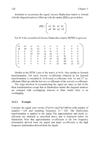
For N=8 the second level Inverse Daubechies matrix DITM2 is given as

a3 b3 a1 b1 0 0 0 0 0 0
a4 b4 a2 b2 0 0 0 0 0 0
0 0 a3 b3 a1 b1 0 0 0 0
0 0 a4 b4 a2 b2 0 0 0 0
0 0 0 0 a3 b3 a1 B1 0 0
0 0 0 0 a4 b4 a2 B2 0 0
0 0 0 0 0 0 a3 B3 a1 b1
0 0 0 0 0 0 a4 B4 a2 b2

Similar to the DTM 1,size of the matrix is 8x10. Also similar to forward
transformation, 1x8 sized wavelet co-efficients obtained in the forward
nd
transformation is extended to 1x10-sized co-efficients with 1st and 2 co-
efficients filled up with the last two co-efficients of the wavelet co-efficients.
The steps involved in reconstructing the signal are same as that of the
Haar transformation except that in Daubechies matrix the diagonal matrices
are arranged with overlapping whereas in Haar matrix there is no
overlapping.

14.2.1 Example

Consider the signal x(n) =a=sin (2*pi*n)+sin(2*pi*100*n) with number of
samples = 128 and sampling frequency Fs = 128. The Daubechies
transformation is applied to the signal The approximation and detail co-
efficients are obtained as described above and is displayed below for
illustration. Note that approximation co-efficients is the low frequency
information derived from the signal and detail co-efficients is the high
frequency information derived from the signal.