Page 22 - Algorithm Collections for Digital Signal Processing Applications using MATLAB

10 Chapter 1

2.1 Roulette Wheel Selection Rule

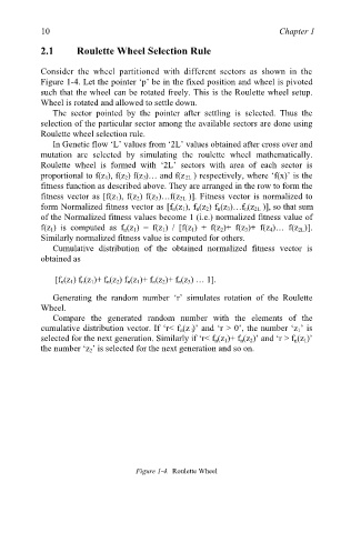
Consider the wheel partitioned with different sectors as shown in the
Figure 1-4. Let the pointer ‘p’ be in the fixed position and wheel is pivoted

such that the wheel can be rotated freely. This is the Roulette wheel setup.
Wheel is rotated and allowed to settle down.

The sector pointed by the pointer after settling is selected. Thus the
selection of the particular sector among the available sectors are done using

Roulette wheel selection rule.
In Genetic flow ‘L’ values from ‘2L’ values obtained after cross over and

mutation are selected by simulating the roulette wheel mathematically.
Roulette wheel is formed with ‘2L’ sectors with area of each sector is
proportional to f(z 1), f(z 2) f(z 3 )… and f(z 2L ) respectively, where ‘f(x)’ is the
fitness function as described above. They are arranged in the row to form the
fitness vector as [f(z 1), f(z 2) f(z 3)…f(z 2L )]. Fitness vector is normalized to
form Normalized fitness vector as [f n(z 1), f n(z 2) f n(z 3)…f n(z 2L )], so that sum
of the Normalized fitness values become 1 (i.e.) normalized fitness value of
f(z 1) is computed as f n(z 1) = f(z 1) / [f(z 1) + f(z 2)+ f(z 3)+ f(z 4)… f(z 2L)].
Similarly normalized fitness value is computed for others.
Cumulative distribution of the obtained normalized fitness vector is
obtained as

[f n(z 1) f n(z 1)+ f n(z 2) f n(z 1)+ f n(z 2)+ f n(z 3) … 1].

Generating the random number ‘r’ simulates rotation of the Roulette
Wheel.
Compare the generated random number with the elements of the
cumulative distribution vector. If ‘r< f n(z 1 )’ and ‘r > 0’, the number ‘z 1’ is
selected for the next generation. Similarly if ‘r< f n(z 1)+ f n(z 2)’ and ‘r > f n(z 1)’
the number ‘z 2’ is selected for the next generation and so on.

Figure 1-4. Roulette Wheel