Page 83 - Algorithm Collections for Digital Signal Processing Applications using MATLAB

2. Probability and Random Process 71

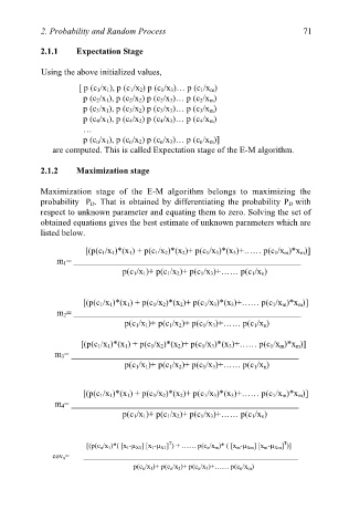
2.1.1 Expectation Stage

Using the above initialized values,

[ p (c 1/x 1), p (c 1/x 2) p (c 1/x 3)… p (c 1/x m)
p (c 2/x 1), p (c 2/x 2) p (c 2/x 3)… p (c 2/x m)
p (c 3/x 1), p (c 3/x 2) p (c 3/x 3)… p (c 3/x m)
p (c 4/x 1), p (c 4/x 2) p (c 4/x 3)… p (c 4/x m)
…
p (c n/x 1), p (c n/x 2) p (c n/x 3)… p (c n/x m)]
are computed. This is called Expectation stage of the E-M algorithm.

2.1.2 Maximization stage

Maximization stage of the E-M algorithm belongs to maximizing the
probability P D. That is obtained by differentiating the probability P D with
respect to unknown parameter and equating them to zero. Solving the set of
obtained equations gives the best estimate of unknown parameters which are
listed below.

[(p(c 1/x 1)*(x 1) + p(c 1/x 2)*(x 2)+ p(c 1/x 3)*(x 3)+…… p(c 1/x m)*x m)]
m 1= ____________________________________________________
p(c 1/x 1)+ p(c 1/x 2)+ p(c 1/x 3)+…… p(c 1/x n)

[(p(c 1/x 1)*(x 1) + p(c 1/x 2)*(x 2)+ p(c 1/x 3)*(x 3)+…… p(c 1/x m)*x m)]
m 2= ____________________________________________________
p(c 1/x 1)+ p(c 1/x 2)+ p(c 1/x 3)+…… p(c 1/x n)

[(p(c 1/x 1)*(x 1) + p(c 1/x 2)*(x 2)+ p(c 1/x 3)*(x 3)+…… p(c 1/x m)*x m)]
m 3= ____________________________________________________
p(c 1/x 1)+ p(c 1/x 2)+ p(c 1/x 3)+…… p(c 1/x n)

[(p(c 1/x 1)*(x 1) + p(c 1/x 2)*(x 2)+ p(c 1/x 3)*(x 3)+…… p(c 1/x m)*x m)]
m 4= ____________________________________________________
p(c 1/x 1)+ p(c 1/x 2)+ p(c 1/x 3)+…… p(c 1/x n)

T
T
[(p(c n /x 1 )*( [x 1 -μ X1 ] [x 1 -μ X1 ] ) + …… p(c n /x m )* ( [x m -μ Xm ] [x m -μ Xm ] )]
cov n = ____________________________________________________________
p(c n /x 1 )+ p(c n /x 2 )+ p(c n /x 3 )+…… p(c n /x m )