Page 196 -

170 Chapter 4 ■ Grey-Level Segmentation

4.5 Cluster-Based Thresholds

The prior discussion of the use of the grey levels on edge pixels to build
local thresholds leads naturally to a discussion of the role of distance
and local geometry in determining thresholds [Kwon, 2004]. Kwon suggests
the use of a cluster-analysis technique to group the pixels into foreground
and background based on a threshold and geometric distances. In particular,
vectors that represent the mean of the two classes are created by scanning the
image with a trial threshold, t. Then the sum of the squared distances between
the class mean and each pixel in the class is computed and used as a significant
part of an objective function J(t) to be minimized. This function is computed
for all values of t and the threshold corresponding to the smallest value of J.
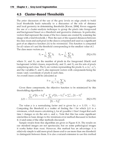
The class mean vectors are:
1 1
v 1 = x k v 2 = x k (EQ 4.53)
N 1 N 2
x k ∈X 1 x k ∈X 2
where N 1 and N 2 are the number of pixels in the foreground (black) and
background (white) classes, respectively, and X 1 and X 2 are the sets of pixels
2
1
comprising each class. The x k are vectors representing the pixels: x k = (x k , x k ),
and the variables v 1 and v 2 also represent vectors with components being the
mean i and j coordinate of pixels in each class.
An overall mean could be calculated as
1
v = x k (EQ 4.54)
N 1 + N 2
x k ∈X
Given these components, the objective function to be minimized by this
thresholding algorithm is:

( ( 2 ( ( 2 ( ( 2

2
p x 1 − v 1 ( + p x 2 − v 2 ( + ( v i − v (
2(
i = 1
2(
x k ∈X 1 x k ∈X 1
J k (t) = (EQ 4.55)
( ( 2
v 1 − v 2
( (
The value p is a normalizing factor and is given by p = 1/(N 1 + N 2 ).
Computing the threshold is a matter of finding the t for which J k (t) is a
minimum, which means calculating J k for all possible t. Don’t forget that each
time t changes so do the sets x 1 and x 2 . Note that this has some significant
similarities in basic design to the minimum error method discussed in Section
4.1.6 and some of the other methods discussed.
Sample results from this algorithm are given in Figure 4.16. The results on
our standard images are not spectacular, but on some pathological images
it works better than most. However, this method has an advantage: it is
relatively simple to add more pixel classes and to use more than one threshold
to distinguish between them. It is also a natural extension to use this method