Page 378 - Applied Numerical Methods Using MATLAB

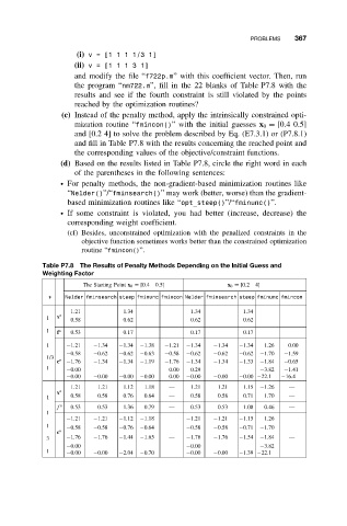
PROBLEMS 367
(i) v=[1111/3 1]
(ii) v=[11131]
and modify the file “f722p.m” with this coefficient vector. Then, run
the program “nm722.m”, fill in the 22 blanks of Table P7.8 with the
results and see if the fourth constraint is still violated by the points
reached by the optimization routines?
(c) Instead of the penalty method, apply the intrinsically constrained opti-
mization routine “fmincon()” with the initial guesses x 0 = [0.40.5]
and [0.2 4] to solve the problem described by Eq. (E7.3.1) or (P7.8.1)
and fill in Table P7.8 with the results concerning the reached point and
the corresponding values of the objective/constraint functions.
(d) Based on the results listed in Table P7.8, circle the right word in each
of the parentheses in the following sentences:
ž For penalty methods, the non-gradient-based minimization routines like
“Nelder()”/“fminsearch()” may work (better, worse) than the gradient-
based minimization routines like “opt_steep()”/“fminunc()”.
ž If some constraint is violated, you had better (increase, decrease) the
corresponding weight coefficient.
(cf) Besides, unconstrained optimization with the penalized constraints in the
objective function sometimes works better than the constrained optimization
routine “fmincon()”.

Table P7.8 The Results of Penalty Methods Depending on the Initial Guess and
Weighting Factor
The Starting Point x 0 = [0.4 0.5] x 0 = [0.2 4]
v Nelder fminsearch steep fminunc fmincon Nelder fminsearch steep fminunc fmincon
1.21 1.34 1.34 1.34
1 x o 0.58 0.62 0.62 0.62
1 f o 0.53 0.17 0.17 0.17
1 −1.21 −1.34 −1.34 −1.38 −1.21 −1.34 −1.34 −1.34 1.26 0.00
−0.58 −0.62 −0.62 −0.63 −0.58 −0.62 −0.62 −0.62 −1.70 −1.59
1/3
c o −1.76 −1.34 −1.34 −1.19 −1.76 −1.34 −1.34 −1.33 −1.84 −0.65
1 −0.00 0.00 0.29 −3.82 −1.41
−0.00 −0.00 −0.00 −0.00 0.00 −0.00 −0.00 −0.00 −22.1 −16.4
1.21 1.21 1.12 1.18 — 1.21 1.21 1.15 −1.26 —
x o
1 0.58 0.58 0.76 0.64 — 0.58 0.58 0.71 1.70 —
f o 0.53 0.53 1.36 0.79 — 0.53 0.53 1.08 0.46 —
1
−1.21 −1.21 −1.12 −1.18 −1.21 −1.21 −1.15 1.26
1 −0.58 −0.58 −0.76 −0.64 −0.58 −0.58 −0.71 −1.70
c o
3 −1.76 −1.76 −1.44 −1.65 — −1.76 −1.76 −1.54 −1.84 —
−0.00 −0.00 −3.82
1 −0.00 −0.00 −2.04 −0.70 −0.00 −0.00 −1.39 −22.1