Page 142 - Autonomous Mobile Robots
P. 142

Data Fusion via Kalman Filter                              125

                                            (a)           Estimation error
                                                 4
                                                                        Q=10
                                               y (m)  2

                                                 0
                                                  0      50     100     150
                                                 4
                                                                         Q=1
                                               y (m)  2

                                                 0
                                                  0      50     100     150
                                                 4
                                                                        Q=
                                                                              0.1
                                               y (m)  2
                                                 0
                                                  0      50     100     150
                                                 4
                                                                       Q=0.01
                                               y (m)  2

                                                 0
                                                  0      50     100     150
                                                 4
                                                                      Q=0.001
                                               y (m)  2

                                                 0
                                                  0      50     100     150
                                                            Time, t (sec)

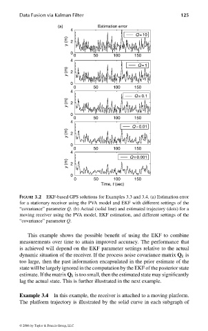
                              FIGURE 3.2 EKF-based GPS solutions for Examples 3.3 and 3.4. (a) Estimation error
                              for a stationary receiver using the PVA model and EKF with different settings of the
                              “covariance” parameter Q. (b) Actual (solid line) and estimated trajectory (dots) for a
                              moving receiver using the PVA model, EKF estimation, and different settings of the
                              “covariance” parameter Q.


                                 This example shows the possible benefit of using the EKF to combine
                              measurements over time to attain improved accuracy. The performance that
                              is achieved will depend on the EKF parameter settings relative to the actual
                              dynamic situation of the receiver. If the process noise covariance matrix Q k is
                              too large, then the past information encapsulated in the prior estimate of the
                              state will be largely ignored in the computation by the EKF of the posterior state
                              estimate. If the matrix Q k is too small, then the estimated state may significantly
                              lag the actual state. This is further illustrated in the next example.

                              Example 3.4  In this example, the receiver is attached to a moving platform.
                              The platform trajectory is illustrated by the solid curve in each subgraph of


                              © 2006 by Taylor & Francis Group, LLC


                                FRANKL: “dk6033_c003” — 2006/3/31 — 16:42 — page 125 — #27
   137   138   139   140   141   142   143   144   145   146   147