Page 284 - Autonomous Mobile Robots

Adaptive Control of Mobile Robots 271

Y y b
2P
v
u
y
2L

x b

O x X

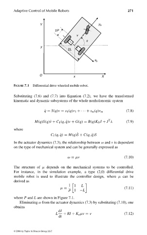
FIGURE 7.1 Differential drive wheeled mobile robot.

Substituting (7.6) and (7.7) into Equation (7.2), we have the transformed
kinematic and dynamic subsystems of the whole nonholonomic system

˙ q = S(q)v = s 1 (q)v 1 + ··· + s m (q)v m (7.8)

T
M(q)S(q)˙v + C 1 (q, ˙q)v + G(q) = B(q)K N I + J λ (7.9)
where
˙
C 1 (q, ˙q) = M(q)S + C(q, ˙q)S
In the actuator dynamics (7.3), the relationship between ω and v is dependent
on the type of mechanical system and can be generally expressed as

ω = µv (7.10)

The structure of µ depends on the mechanical systems to be controlled.
For instance, in the simulation example, a type (2,0) differential drive
mobile robot is used to illustrate the controller design, where µ can be
derived as

1 1 L
µ = (7.11)
P 1 −L
where P and L are shown in Figure 7.1.
Eliminating ω from the actuator dynamics (7.3) by substituting (7.10), one
obtains
dI
L + RI + K a µv = ν (7.12)
dt

© 2006 by Taylor & Francis Group, LLC

FRANKL: “dk6033_c007” — 2006/3/31 — 16:43 — page 271 — #5