Page 29 - Autonomous Mobile Robots

Visual Guidance for Autonomous Vehicles 13

camera and its intrinsic parameters. We can rewrite (1.1) as:

˜
x = K[R T]X: K ∈ R 3×3 , R ∈ SO(3), T ∈ R 3 (1.2)
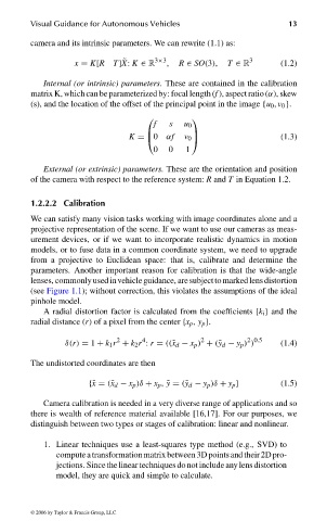
Internal (or intrinsic) parameters. These are contained in the calibration
matrix K, which can be parameterized by: focal length (f ), aspect ratio (α), skew
(s), and the location of the offset of the principal point in the image {u 0 , v 0 }.

 
f s u 0
K = 0 αf v 0 (1.3)


0 0 1
External (or extrinsic) parameters. These are the orientation and position
of the camera with respect to the reference system: R and T in Equation 1.2.

1.2.2.2 Calibration

We can satisfy many vision tasks working with image coordinates alone and a
projective representation of the scene. If we want to use our cameras as meas-
urement devices, or if we want to incorporate realistic dynamics in motion
models, or to fuse data in a common coordinate system, we need to upgrade
from a projective to Euclidean space: that is, calibrate and determine the
parameters. Another important reason for calibration is that the wide-angle
lenses, commonlyusedinvehicleguidance, aresubjecttomarkedlensdistortion
(see Figure 1.1); without correction, this violates the assumptions of the ideal
pinhole model.
A radial distortion factor is calculated from the coefficients {k i } and the
radial distance (r) of a pixel from the center {x p , y p }.
2
4
2 0.5
2
δ(r) = 1 + k 1 r + k 2 r : r = ((˜x d − x p ) + (˜y d − y p ) ) (1.4)
The undistorted coordinates are then
{˜x = (˜x d − x p )δ + x p , ˜y = (˜y d − y p )δ + y p } (1.5)

Camera calibration is needed in a very diverse range of applications and so
there is wealth of reference material available [16,17]. For our purposes, we
distinguish between two types or stages of calibration: linear and nonlinear.

1. Linear techniques use a least-squares type method (e.g., SVD) to
computeatransformationmatrixbetween3Dpointsandtheir2Dpro-
jections. Since the linear techniques do not include any lens distortion
model, they are quick and simple to calculate.

© 2006 by Taylor & Francis Group, LLC

FRANKL: “dk6033_c001” — 2006/3/31 — 16:42 — page 13 — #13