Page 288 - Autonomous Mobile Robots

Adaptive Control of Mobile Robots 275

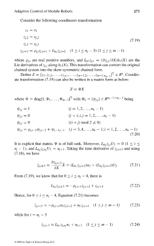
Consider the following coordinates transformation

z 1 = x 1

z j,2 = x j,2
(7.19)
z j,3 = x j,3
z
z j,i+3 = ρ j,i z j,i+1 + L h 1 j,i+2 (1 ≤ i ≤ n j − 3)(1 ≤ j ≤ m − 1)
where ρ j,i are real positive numbers, and L h1 z j,i = (∂z j,i /∂X)h 1 (X) are the
Lie derivatives of z j,i along h 1 (X). This transformation can convert the original
chained system into the skew-symmetric chained form.
T
n
] ∈ R . Coordin-
Define Z =[z 1 , z 1,2 , ... , z 1,n 1 , ... , z m−1,2 , ... , z m−1,n m−1
ate transformation (7.19) can also be written in a matrix form as below:
Z = X
T
where = diag[1, 1 , ... , m−1 ] with k =[ψ j,i ]∈ R n k −1×n k −1 being
ψ j,j = 1 (j = 1, 2, ... , n k − 1)
ψ j,i = 0 (j < i; i, j = 1, 2, ... , n k − 1)
ψ j,i = 0 ((i + j) mod 2 = 0)

ψ j,i = ρ j,i−3 ψ j,i−2 + ψ j−1,i−1 ( j = 3, 4, ... , n k − 1; i = 1, 2, ... , n k − 1)
(7.20)

z
It is explicit that matrix is of full rank. Moreover, L h 2 j,i U 2 = 0 (1 ≤ i ≤
z U 2 = u j+1 . Taking the time derivative of z j,i+3 and using
n j − 1), and L h 2 j,n j
(7.18), we have
∂z j,i+3
z
˙
z
˙ z j,i+3 = X = (L h 1 j,i+3 )u 1 + (L h 2 j,i+3 )U 2 (7.21)
∂X
From (7.19), we know that for 0 ≤ i ≤ n j − 4, there is
z
L h 1 j,i+3 =−ρ j,i+1 z j,i+2 + z j,i+4 (7.22)
Hence, for 0 ≤ i ≤ n j − 4, Equation (7.21) becomes

˙ z j,i+3 =−ρ j,i+1 u 1 z j,i+2 + u 1 z j,i+4 (1 ≤ j ≤ m − 1) (7.23)

while for i = n j − 3

z u (1 ≤ j ≤ m − 1) (7.24)
˙ z j,i+3 = L h 1 j,n j 1 + u j+1

© 2006 by Taylor & Francis Group, LLC

FRANKL: “dk6033_c007” — 2006/3/31 — 16:43 — page 275 — #9