Page 188 - Basic Structured Grid Generation

Variational methods and adaptive grid generation 177

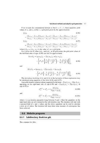
If we re-scale the computational domain so that h = k = 1, these equations yield
values of f x and f y at the i, j grid point given by the approximations

[f x ] ij (6.96)
(f i+1,j − f i−1,j )(y i,j+1 − y i,j−1 ) − (f i,j+1 − f i,j−1 )(y i+1,j − y i−1,j )
= ,
(x i+1,j − x i−1,j )(y i,j+1 − y i,j−1 ) − (x i,j+1 − x i,j−1 )(y i+1,j − y i−1,j )
[f y ] ij (6.97)
(f i,j+1 − f i,j−1 )(x i+1,j − x i−1,j ) − (f i+1,j − f i−1,j )(x i,j+1 − x i,j−1 )
= ,
(x i+1,j − x i−1,j )(y i,j+1 − y i,j−1 ) − (x i,j+1 − x i,j−1 )(y i+1,j − y i−1,j )
where [f ] ij = f(x ij ,y ij ) is the value of z at a grid point.
For a given set of values [x] i,j and [y] i,j at all grid points, the grid point values of
the left-hand sides of eqns (6.94) can now be approximated:

[L(x)] ij =[g 22 x ξξ ] ij −[2g 12 x ξη ] ij +[g 11 x ηη ] ij
2
√ ∂ 1 + (f y ) ∂ f x f y
2
− J γ √ − √ (6.98)
∂x γ ∂y γ
ij
and
[L(y)] ij =[g 22 y ξξ ] ij −[2g 12 y ξη ] ij +[g 11 y ηη ] ij
2
√ ∂ f x f y ∂ 1 + (f x )
2
− J γ − √ + √ . (6.99)
∂x γ ∂y γ
ij
The derivatives involving ∂/∂x and ∂/∂y in the last terms of these expressions may
be calculated using equations of the form (6.96) and (6.97).
A possible iterative solution scheme suggested by the terms −2[g 22 ] ij x i,j −2[g 11 ] ij x i,j
appearing on the right-hand side of eqn (6.98) and −2[g 22 ] ij y i,j − 2[g 11 ] ij y i,j in
eqn (6.99) is
m+1 m [L(x)] ij
x = x + σ (6.100)
i,j i,j
2[g 22 + g 11 ] ij
and
y m+1 = y m + σ [L(y)] ij , (6.101)
i,j i,j
2[g 22 + g 11 ] ij
where σ is an iteration parameter lying between 0 and 1. Here the quantities on the
right-hand sides are all evaluated at the mth iteration step. The iteration will start with
aguessedfieldof x and y values, and the above equations can be used to calculate
a new set of values. The iteration will stop when some measure of convergence has
been achieved.

6.6 Website programs

6.6.1 Subdirectory: Book/var.gds

This contains five files: