Page 205 - Basic Structured Grid Generation

194 Basic Structured Grid Generation

x 5 x 4
x 1
x 3
x 6
x 2

Fig. 8.6 New Delaunay triangulation.

x 4

x 5

x 3

x 6 x 9 x
x 8 2

x 7 x 1

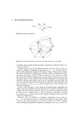
Fig. 8.7 New Delaunay triangulation with removal of four edges and creation of seven edges.

tessellation, and new edges are then created by connecting x 6 to the four vertices of S,
as shown in Fig. 8.6.
Another example of the Bowyer-Watson procedure is shown in Fig. 8.7, where we
start from a Delaunay triangulation of eight points x 1 , x 2 ,.. . , x 8 . To reduce the com-
plexity of the diagram this example has been given a degree of degeneracy, in that x 5
lies on the circumcircle of triangle x 2 x 3 x 4 . In other words the circumcircles of trian-
gles x 2 x 3 x 4 and x 2 x 4 x 5 coincide. The new data point x 9 is now found to lie within
the circumcircles of the five triangles x 2 x 3 x 4 , x 2 x 4 x 5 (which coincide), x 1 x 2 x 8 , x 5 x 6 x 8 ,
and x 5 x 2 x 8 .The set S thus consists of the (non-convex) polygon x 1 x 2 x 3 x 4 x 5 x 6 x 8 ,and
removal of internal edges implies removal of the connections x 2 x 8 , x 2 x 4 , x 2 x 5 ,and
x 5 x 8 . The large hole created in the triangulation is then filled with connections from
x 9 to the points x 1 , x 2 , x 3 , x 4 , x 5 , x 6 ,and x 8 (dotted lines as shown), giving a new
Delaunay triangulation.
In case 2, the new point x i+1 lies outside the existing Delaunay triangulation but
within at least one circumcircle. We can define the set S as before as the union of the
triangles whose circumcircles contain x i+1 , but now we remove those edges in S which
are nearest to (and ‘visible’ from) x i+1 . The new Delaunay triangulation is obtained
by connecting x i+1 to all the vertices of the triangles composing S and to any other
vertex of T i visible from x i+1 .
Figure 8.8 shows an example of a Delaunay triangulation of five points x 1 ,
x 2 ,..., x 5 . A new data point x 6 lies within the circumcircle of triangle x 1 x 2 x 5 ,which
is the set S. The edge connecting x 1 to x 2 is the one visible to x 6 , and this is deleted.
The next Delaunay triangulation is obtained by connecting x 6 to x 1 , x 5 , x 2 ,and also x 3 .