Page 50 - Basic Structured Grid Generation

Classical differential geometry of space-curves 39

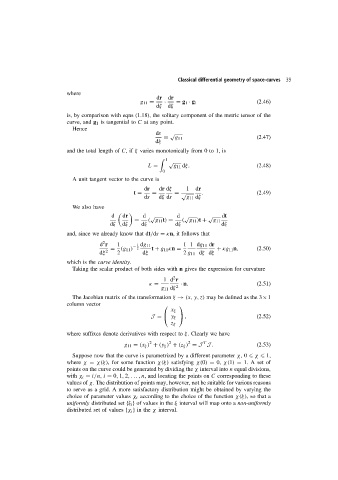
where
dr dr
g 11 = · = g 1 · g 1 (2.46)
dξ dξ
is, by comparison with eqns (1.18), the solitary component of the metric tensor of the
curve, and g 1 is tangential to C at any point.
Hence
ds √
= g 11 (2.47)
dξ
and the total length of C,if ξ varies monotonically from 0 to 1, is

1
√
L = g 11 dξ. (2.48)
0
A unit tangent vector to the curve is
dr dr dξ 1 dr
t = = = √ . (2.49)
ds dξ ds g 11 dξ
We also have
d dr d √ d √ √ dt
= ( g 11 t) = ( g 11 )t + g 11
dξ dξ dξ dξ dξ
and, since we already know that dt/ds = κn, it follows that
2
d r 1 1 dg 11 1 1 dg 11 dr
= (g 11 ) − 2 t + g 11 κn = + κg 11 n, (2.50)
dξ 2 2 dξ 2 g 11 dξ dξ
which is the curve identity.
Taking the scalar product of both sides with n gives the expression for curvature
2
1 d r
κ = · n. (2.51)
g 11 dξ 2
The Jacobian matrix of the transformation ξ → (x,y,z) maybedefinedasthe 3×1
column vector
 
x ξ
J =  y ξ  , (2.52)
z ξ
where suffixes denote derivatives with respect to ξ. Clearly we have
2
2
2
T
g 11 = (x ξ ) + (y ξ ) + (z ξ ) = J J . (2.53)
Suppose now that the curve is parametrized by a different parameter χ,0 χ 1,
where χ = χ(ξ), for some function χ(ξ) satisfying χ(0) = 0, χ(1) = 1. A set of
points on the curve could be generated by dividing the χ interval into n equal divisions,
with χ i = i/n, i = 0, 1, 2,. ..,n, and locating the points on C corresponding to these
values of χ. The distribution of points may, however, not be suitable for various reasons
to serve as a grid. A more satisfactory distribution might be obtained by varying the
choice of parameter values χ i according to the choice of the function χ(ξ),sothata
uniformly distributed set {ξ i } of values in the ξ interval will map onto a non-uniformly
distributed set of values {χ i } in the χ interval.