Page 85 - Basics of MATLAB and Beyond

clf
gplot(A,[x y])
axis off

(Try zooming in on this plot by typing zoom and dragging the mouse.)
The adjacency matrix here (A) is a 4251×4253 sparse matrix with 12,289
non-zero elements, occupying 164 kB of storage. A full matrix of this
size would require 145 MB.
(From now on in this book, the clf command will be omitted from
the examples; you will need to supply your own clfs where appropriate.)

25.2 Example: Communication Network

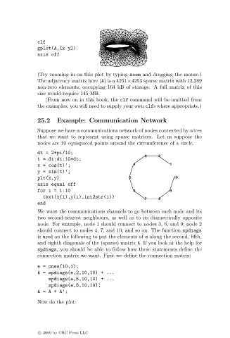
Suppose we have a communications network of nodes connected by wires
that we want to represent using sparse matrices. Let us suppose the
nodes are 10 equispaced points around the circumference of a circle.
dt = 2*pi/10;
t = dt:dt:10*dt;
x = cos(t)’;
y = sin(t)’;
plt(x,y)
axis equal off
for i = 1:10
text(x(i),y(i),int2str(i))
end
We want the communications channels to go between each node and its
two second-nearest neighbours, as well as to its diametrically opposite
node. For example, node 1 should connect to nodes 3, 6, and 9; node 2
should connect to nodes 4, 7, and 10; and so on. The function spdiags
is used on the following to put the elements of e along the second, fifth,
and eighth diagonals of the (sparse) matrix A. If you look at the help for
spdiags, you should be able to follow how these statements define the
connection matrix we want. First we define the connection matrix:

e = ones(10,1);
A = spdiags(e,2,10,10) + ...
spdiags(e,5,10,10) + ...
spdiags(e,8,10,10);
A=A+A’;

Now do the plot:

c 2000 by CRC Press LLC