Page 120 - Biomimetics : Biologically Inspired Technologies

Bar-Cohen : Biomimetics: Biologically Inspired Technologies DK3163_c003 Final Proof page 106 21.9.2005 11:40pm

106 Biomimetics: Biologically Inspired Technologies

eventually led to the realization that the control of movement and the control of thought are
implemented in essentially the same manner; using the same cortical and subcortical structures
(indeed, the theory postulates that there are many combined movement and thought processes
which are represented as unitized symbols at higher levels in the action hierarchy — e.g., a back
dive action routine in which visual perception must feed corrections to the movement control in
order to enter the water vertically).
To see what attractor networks of this unusual type are all about, the reader is invited to pause in
their reading and build (e.g., using C, LabVIEW, MATLAB, etc.) a simple working example using
the following prescription. If you accept this invitation, you will see first-hand the amazing
capabilities of these networks (which will help you appreciate and accept the theory). While
simple, this network possesses many of the important behavioral characteristics of the hypothesized
design of biological feature attractor modules.
We will use two N-dimensional real column vectors, x and y, to represent the states of N
neurons in each of two ‘‘neural fields.’’ For good results, N should be at least 10,000 (even better
results are obtained for N above 30,000). Using a good random number generator, create L pairs
of x and y vectors {(x 1 ,y 1 ), (x 2 ,y 2 ), .. ., (x L ,y L )} with each x i vector and each y i vector having
binary (0 and 1) entries selected independently at random; where the probability of each compon-
ent being 1 is p. Use, for example, p ¼ 0.003 and L ¼ 5,000 for N ¼ 20,000. As you will see,
these x i and y i pairs turn out to be stable states of the network. Each x k and y k vector pair, k ¼ 1,
2, ... , L represents one of the L symbols of the network. For simplicity, we will concentrate
on the x k vector as the representation of symbol k. Thus, each symbol is represented
by a collection of about Np ‘‘active’’ neurons. The random selection of the symbol neuron sets
and the deliberate processes of neuronal interconnection between the sets correspond to the
development and refinement processes in each thalamocortical module that are described later in
this section.
During development of the bipartite stable states {(x 1 ,y 1 ), (x 2 ,y 2 ), . .., (x L ,y L )} (which happens
gradually over time in biology, but all at once in this simple model), connections between the
neurons of the x and y fields are also established. These connections are very simple: each neuron of
x k (i.e., the neurons of the x field whose indices within x k have a 1 assigned to them) sends a
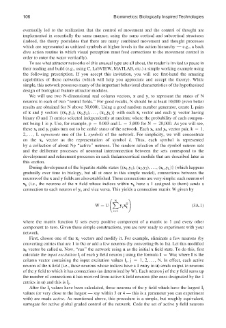
connection to each neuron of y k and vice versa. This yields a connection matrix W given by
!
X
N
W ¼ U y x T (3A:1)
k k
i¼1
where the matrix function U sets every positive component of a matrix to 1 and every other
component to zero. Given these simple constructions, you are now ready to experiment with your
network.
First, choose one of the x k vectors and modify it. For example, eliminate a few neurons (by
converting entries that are 1 to 0s) or add a few neurons (by converting 0s to 1s). Let this modified
x k vector be called u. Now, ‘‘run’’ the network using u as the initial x field state. To do this, first
calculate the input excitation I j of each y field neuron j using the formula I ¼ Wu; where I is the
column vector containing the input excitation values I j ,j ¼ 1, 2, . . . , N. In effect, each active
neuron of the x field (i.e., those neurons whose indices have a 1 entry in u) sends output to neurons
of the y field to which it has connections (as determined by W). Each neuron j of the y field sums up
the number of connections it has received from active x field neurons (the ones designated by the 1
entries in u) and this is I j .
After the I j values have been calculated, those neurons of the y field which have the largest I j
values (or very close to the largest — say within 3 or 4 — this is a parameter you can experiment
with) are made active. As mentioned above, this procedure is a simple, but roughly equivalent,
surrogate for active global graded control of the network. Code the set of active y field neurons