Page 98 - Calculus Demystified

CHAPTER 3 Applications of the Derivative
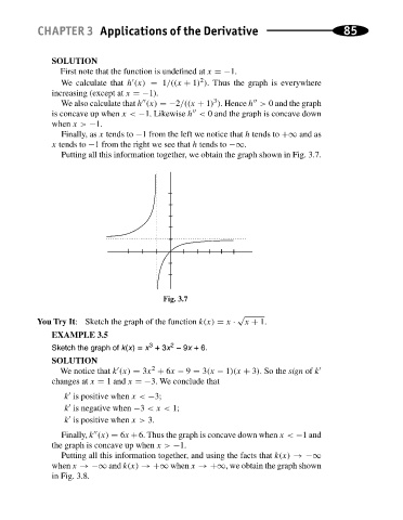
SOLUTION 85
First note that the function is undefined at x =−1.
2
We calculate that h (x) = 1/((x + 1) ). Thus the graph is everywhere

increasing (except at x =−1).
3

We also calculate that h (x) =−2/((x + 1) ). Hence h > 0 and the graph

is concave up when x< −1. Likewise h < 0 and the graph is concave down
when x> −1.
Finally, as x tends to −1 from the left we notice that h tends to +∞ and as
x tends to −1 from the right we see that h tends to −∞.
Putting all this information together, we obtain the graph shown in Fig. 3.7.

Fig. 3.7

√
You Try It: Sketch the graph of the function k(x) = x · x + 1.
EXAMPLE 3.5
3
2
Sketch the graph of k(x) = x + 3x − 9x + 6.
SOLUTION
2

We notice that k (x) = 3x + 6x − 9 = 3(x − 1)(x + 3).Sothe sign of k
changes at x = 1 and x =−3. We conclude that

k is positive when x< −3;

k is negative when −3 <x < 1;
k is positive when x> 3.

Finally, k (x) = 6x +6. Thus the graph is concave down when x< −1 and
the graph is concave up when x> −1.
Putting all this information together, and using the facts that k(x) →−∞
when x →−∞ and k(x) →+∞ when x →+∞, we obtain the graph shown
in Fig. 3.8.