Page 210 - Classification Parameter Estimation & State Estimation An Engg Approach Using MATLAB

FEATURE SELECTION 199

in step 3. This loop also controls the order in which branches are
explored. Both aspects influence the computational efficiency of the
algorithm. In Figure 6.4, the list of indices of elements that are deleted
from a node to form the child nodes follows a specific pattern (see
exercise 2). The indices of these elements are shown in the figure. Note
that this tree is not minimal because some twigs have their leaves at a
level higher than D. Of course, pruning these useless twigs in advance is
computationally more efficient.

6.2.2 Suboptimal search

Although the branch-and-bound algorithm can save many calculations
relative to an exhaustive search (especially for large values of q(D)), it
may still require too much computational effort.
Another possible defect of branch-and-bound is the top-down search
order. It starts with the full set of measurements and successively deletes
elements. However, the assumption that the performance becomes worse
as the number of features decreases holds true only in theory; see Figure
6.1. In practice, the finite training set may give rise to an overoptimistic
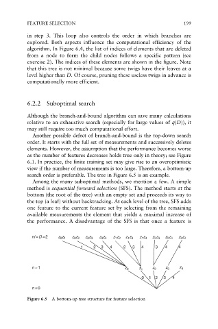
view if the number of measurements is too large. Therefore, a bottom-up
search order is preferable. The tree in Figure 6.5 is an example.
Among the many suboptimal methods, we mention a few. A simple
method is sequential forward selection (SFS). The method starts at the
bottom (the root of the tree) with an empty set and proceeds its way to
the top (a leaf) without backtracking. At each level of the tree, SFS adds
one feature to the current feature set by selecting from the remaining
available measurements the element that yields a maximal increase of
the performance. A disadvantage of the SFS is that once a feature is

nl=D= 2 z z z z z z z z z z z z z z z z z z z z
0 4
1 2
1 3
1 4
3 4
2 4
2 3
0 2
0 1
0 3
1 2 3 4 2 3 4 3 4 4
n = 1 z 0 z 1 z 2 z 3 z 4
0 1 2 3 4
n= 0
Figure 6.5 A bottom-up tree structure for feature selection