Page 145 - Classification Parameter Estimation & State Estimation An Engg Approach Using MATLAB

134 STATE ESTIMATION

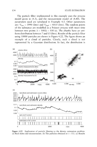
The particle filter implemented in this example uses the process
model given in (4.3), and the measurement model of (4.40). The
parameters used are tabulated in Example 4.5. Other parameters
are: V low ¼ 3990 (litre) and V high ¼ 4010 (litre). The random points
of the substance are modelled as a Poisson process with mean time
between two points ¼ 100 ¼ 100 (s). The chunks have an uni-
form distribution between 7 and 13 (litre). Results of the particle filter
using 10000 particles are shown in Figure 4.22. The figure shows an
example of a cloud of particles. Clearly, such a cloud is not
represented by a Gaussian distribution. In fact, the distribution is

(a) (b)
volume (litre)
4020
volume (litre)
4000 4005
density
0.1
0.09 4000
0.08
volume measurements (litre)
4050
4000
3995
3950
density measurements (V)
0.4
0.2
3990
0
0 2000 i∆(s) 4000 0.094 0.096 density 0.098
(c)
4030 real (thick) and estimated volume (litre)
4020
4010
4000
3990
0.11
real (thick) and estimated density
0.1
0.09
0.08
real on/off control

estimated on/off control

0 2000 i∆(s) 4000

Figure 4.22 Application of particle filtering to the density estimation problem.
(a) Real states and measurements. (b) The particles obtained at i ¼ 511. (c) Results